

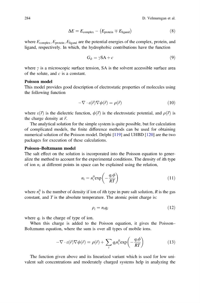
DE ¼ E complex À E protein Ç E ligand
À
Á
ð8Þ
where E complex ; E protein ; E ligand are the potential energies of the complex, protein, and
ligand, respectively. In which, the hydrophobic contributions have the function
G / ¼ cSA þ c
ð9Þ
where c is a microscopic surface tension, SA is the solvent accessible surface area
of the solute, and c is a constant.
Poisson model
This model provides good description of electrostatic properties of molecules using
the following function
Àr Á e ~ r
ð Þr/ ~ r
ð Þ ¼ q ~ r
ð Þ
ð10Þ
where e ~ r
ð Þ is the dielectric function, / ~ r
ð Þ is the electrostatic potential, and q ~ r
ð Þ is
the charge density at ~ r.
The analytical solution for the simple system is quite possible, but for calculation
of complicated models, the finite difference methods can be used for obtaining
numerical solution of the Poisson model. Delphi [119] and UHBD [120] are the two
packages for execution of these calculations.
Poisson–Boltzmann model
The salt effect on the solution is incorporated into the Poisson equation to generalize the method to account for the experimental conditions. The density of ith type
of ion n i at different points in space can be explained using the relation,
n i ¼ n
0
i exp À
q i /
RT
ð11Þ
where n
0
i is the number of density if ion of ith type in pure salt solution, R is the gas
constant, and T is the absolute temperature. The atomic point charge is:
q i ¼ n i q i
ð12Þ
where q i is the charge of type of ion.
When this charge is added to the Poisson equation, it gives the Poisson–
Boltzmann equation, where the sum is over all types of mobile ions.
Àr Á e ~ r
ð Þr/ ~ r
ð Þ ¼ q ~ r
ð Þ þ
X
i
q i n
0
i exp À
q i /
RT
ð13Þ
The function given above and its linearized variant which is used for low univalent salt concentrations and moderately charged systems help in analyzing the
284
D. Velmurugan et al.
À
Á
ð8Þ
where E complex ; E protein ; E ligand are the potential energies of the complex, protein, and
ligand, respectively. In which, the hydrophobic contributions have the function
G / ¼ cSA þ c
ð9Þ
where c is a microscopic surface tension, SA is the solvent accessible surface area
of the solute, and c is a constant.
Poisson model
This model provides good description of electrostatic properties of molecules using
the following function
Àr Á e ~ r
ð Þr/ ~ r
ð Þ ¼ q ~ r
ð Þ
ð10Þ
where e ~ r
ð Þ is the dielectric function, / ~ r
ð Þ is the electrostatic potential, and q ~ r
ð Þ is
the charge density at ~ r.
The analytical solution for the simple system is quite possible, but for calculation
of complicated models, the finite difference methods can be used for obtaining
numerical solution of the Poisson model. Delphi [119] and UHBD [120] are the two
packages for execution of these calculations.
Poisson–Boltzmann model
The salt effect on the solution is incorporated into the Poisson equation to generalize the method to account for the experimental conditions. The density of ith type
of ion n i at different points in space can be explained using the relation,
n i ¼ n
0
i exp À
q i /
RT
ð11Þ
where n
0
i is the number of density if ion of ith type in pure salt solution, R is the gas
constant, and T is the absolute temperature. The atomic point charge is:
q i ¼ n i q i
ð12Þ
where q i is the charge of type of ion.
When this charge is added to the Poisson equation, it gives the Poisson–
Boltzmann equation, where the sum is over all types of mobile ions.
Àr Á e ~ r
ð Þr/ ~ r
ð Þ ¼ q ~ r
ð Þ þ
X
i
q i n
0
i exp À
q i /
RT
ð13Þ
The function given above and its linearized variant which is used for low univalent salt concentrations and moderately charged systems help in analyzing the
284
D. Velmurugan et al.