

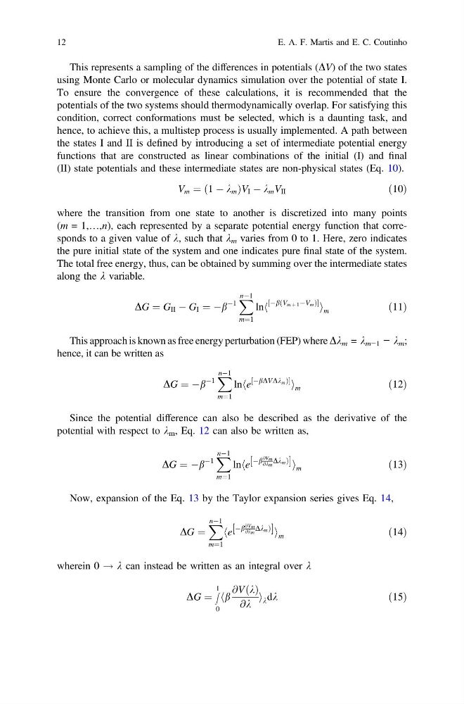
This represents a sampling of the differences in potentials (DV) of the two states
using Monte Carlo or molecular dynamics simulation over the potential of state I.
To ensure the convergence of these calculations, it is recommended that the
potentials of the two systems should thermodynamically overlap. For satisfying this
condition, correct conformations must be selected, which is a daunting task, and
hence, to achieve this, a multistep process is usually implemented. A path between
the states I and II is defined by introducing a set of intermediate potential energy
functions that are constructed as linear combinations of the initial (I) and final
(II) state potentials and these intermediate states are non-physical states (Eq. 10).
V m ¼ 1 À k m
ð
ÞV I À k m V II
ð10Þ
where the transition from one state to another is discretized into many points
(m = 1,…,n), each represented by a separate potential energy function that corresponds to a given value of k, such that k m varies from 0 to 1. Here, zero indicates
the pure initial state of the system and one indicates pure final state of the system.
The total free energy, thus, can be obtained by summing over the intermediate states
along the k variable.
DG ¼ G II À G I ¼ Àb
À1
X nÀ1
m¼1
lnh
Àb V m þ 1 ÀV m
ð
Þ
½
i m
ð11Þ
This approach is known as free energy perturbation (FEP) where Dk m = k m−1 − k m ;
hence, it can be written as
DG ¼ Àb
À1
X nÀ1
m¼1
lnhe
ÀbDVDk m Þ
½
i m
ð12Þ
Since the potential difference can also be described as the derivative of the
potential with respect to k m , Eq. 12 can also be written as,
DG ¼ Àb
À1
X nÀ1
m¼1
lnhe
Àb
@Vm
@km Dk m Þ
½
i m
ð13Þ
Now, expansion of the Eq. 13 by the Taylor expansion series gives Eq. 14,
DG ¼
X nÀ1
m¼1
he
Àb
@Vm
@km Dk m Þ
½
i m
ð14Þ
wherein 0 ! k can instead be written as an integral over k
DG ¼
Z 1
0
hb
@V k
ð Þ
@k
i k dk
ð15Þ
12
E. A. F. Martis and E. C. Coutinho
using Monte Carlo or molecular dynamics simulation over the potential of state I.
To ensure the convergence of these calculations, it is recommended that the
potentials of the two systems should thermodynamically overlap. For satisfying this
condition, correct conformations must be selected, which is a daunting task, and
hence, to achieve this, a multistep process is usually implemented. A path between
the states I and II is defined by introducing a set of intermediate potential energy
functions that are constructed as linear combinations of the initial (I) and final
(II) state potentials and these intermediate states are non-physical states (Eq. 10).
V m ¼ 1 À k m
ð
ÞV I À k m V II
ð10Þ
where the transition from one state to another is discretized into many points
(m = 1,…,n), each represented by a separate potential energy function that corresponds to a given value of k, such that k m varies from 0 to 1. Here, zero indicates
the pure initial state of the system and one indicates pure final state of the system.
The total free energy, thus, can be obtained by summing over the intermediate states
along the k variable.
DG ¼ G II À G I ¼ Àb
À1
X nÀ1
m¼1
lnh
Àb V m þ 1 ÀV m
ð
Þ
½
i m
ð11Þ
This approach is known as free energy perturbation (FEP) where Dk m = k m−1 − k m ;
hence, it can be written as
DG ¼ Àb
À1
X nÀ1
m¼1
lnhe
ÀbDVDk m Þ
½
i m
ð12Þ
Since the potential difference can also be described as the derivative of the
potential with respect to k m , Eq. 12 can also be written as,
DG ¼ Àb
À1
X nÀ1
m¼1
lnhe
Àb
@Vm
@km Dk m Þ
½
i m
ð13Þ
Now, expansion of the Eq. 13 by the Taylor expansion series gives Eq. 14,
DG ¼
X nÀ1
m¼1
he
Àb
@Vm
@km Dk m Þ
½
i m
ð14Þ
wherein 0 ! k can instead be written as an integral over k
DG ¼
Z 1
0
hb
@V k
ð Þ
@k
i k dk
ð15Þ
12
E. A. F. Martis and E. C. Coutinho