

62
S. A. Khan et al.
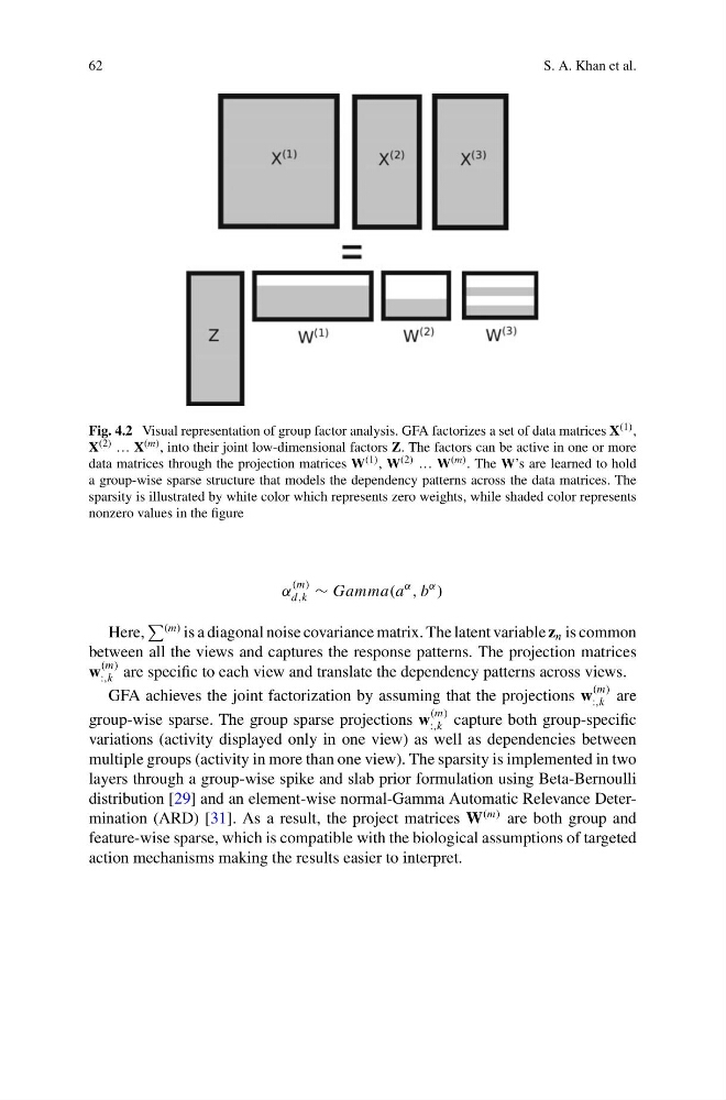
Fig. 4.2 Visual representation of group factor analysis. GFA factorizes a set of data matrices X (1) ,
X (2) … X (m) , into their joint low-dimensional factors Z. The factors can be active in one or more
data matrices through the projection matrices W (1) , W (2) … W (m) . The W’s are learned to hold
a group-wise sparse structure that models the dependency patterns across the data matrices. The
sparsity is illustrated by white color which represents zero weights, while shaded color represents
nonzero values in the figure
α
(m)
d,k ∼ Gamma(a
α
, b
α
)
Here,
(m) is a diagonal noise covariance matrix. The latent variable z n is common
between all the views and captures the response patterns. The projection matrices
w
(m)
:,k are specific to each view and translate the dependency patterns across views.
GFA achieves the joint factorization by assuming that the projections w
(m)
:,k are
group-wise sparse. The group sparse projections w
(m)
:,k capture both group-specific
variations (activity displayed only in one view) as well as dependencies between
multiple groups (activity in more than one view). The sparsity is implemented in two
layers through a group-wise spike and slab prior formulation using Beta-Bernoulli
distribution [29] and an element-wise normal-Gamma Automatic Relevance Determination (ARD) [31]. As a result, the project matrices W
(m) are both group and
feature-wise sparse, which is compatible with the biological assumptions of targeted
action mechanisms making the results easier to interpret.
S. A. Khan et al.
Fig. 4.2 Visual representation of group factor analysis. GFA factorizes a set of data matrices X (1) ,
X (2) … X (m) , into their joint low-dimensional factors Z. The factors can be active in one or more
data matrices through the projection matrices W (1) , W (2) … W (m) . The W’s are learned to hold
a group-wise sparse structure that models the dependency patterns across the data matrices. The
sparsity is illustrated by white color which represents zero weights, while shaded color represents
nonzero values in the figure
α
(m)
d,k ∼ Gamma(a
α
, b
α
)
Here,
(m) is a diagonal noise covariance matrix. The latent variable z n is common
between all the views and captures the response patterns. The projection matrices
w
(m)
:,k are specific to each view and translate the dependency patterns across views.
GFA achieves the joint factorization by assuming that the projections w
(m)
:,k are
group-wise sparse. The group sparse projections w
(m)
:,k capture both group-specific
variations (activity displayed only in one view) as well as dependencies between
multiple groups (activity in more than one view). The sparsity is implemented in two
layers through a group-wise spike and slab prior formulation using Beta-Bernoulli
distribution [29] and an element-wise normal-Gamma Automatic Relevance Determination (ARD) [31]. As a result, the project matrices W
(m) are both group and
feature-wise sparse, which is compatible with the biological assumptions of targeted
action mechanisms making the results easier to interpret.