

4 Matrix and Tensor Factorization Methods …
61
4.2.2 Latent Dirichlet Allocation
The Latent Dirichlet Allocation (LDA [20, 21]) is a probabilistic formulation of
factorization for discrete data sets. Formally, it is a three-level hierarchical Bayesian
model that models the probabilities of each input feature to appear in each component.
The Dirichlet distribution is a multivariate probability distribution used in LDA to
mitigate overfitting and to help LDA to achieve its generalizability beyond the training
data. LDA has demonstrated wide applicability in natural language processing, as
text data sets can directly be encoded as discrete variables [22–24] as well as in
genomic data sets [25–27].
4.2.3 Group Factor Analysis
Group factor analysis (GFA [28, 29]) is a recent machine learning method designed
to capture relationships between multiple data sets. GFA models the relationships as
statistical dependencies by reducing multiple data sets (also known as views) to learn
a joint low-dimensional representation. The joint representation of the data sets is
characterized by components that may be active in one or several of the data views as
shown in Fig. 4.2. An active component captures underlying relationships between
the views in which it is active. For example, the active component of all views captures
a common dependency structure between all views, while a component active only in
a single view identifies the variance and features unique to that particular view only.
GFA learns the components and their activity patterns in a truly data-driven fashion,
making it possible to comprehensively capture the interdependencies between all the
data views. An easy to use implementation of GFA has been made freely available
as an R-package [30].
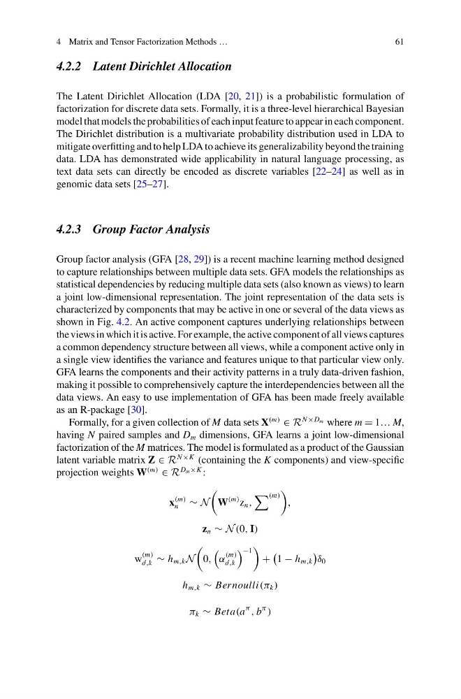
Formally, for a given collection of M data sets X
(m)
∈ R
N ×D m where m = 1… M,
having N paired samples and D m dimensions, GFA learns a joint low-dimensional
factorization of the M matrices. The model is formulated as a product of the Gaussian
latent variable matrix Z ∈ R
N ×K (containing the K components) and view-specific
projection weights W
(m)
∈ R
D m ×K :
x
(m)
n
∼ N
W
(m) z n ,
(m)
,
z n ∼ N (0, I)
w
(m)
d,k ∼ h m,k N
0,
α
(m)
d,k
−1
+
1 − h m,k
δ 0
h m,k ∼ Bernoulli(π k )
π k ∼ Beta(a
π
, b
π
)
61
4.2.2 Latent Dirichlet Allocation
The Latent Dirichlet Allocation (LDA [20, 21]) is a probabilistic formulation of
factorization for discrete data sets. Formally, it is a three-level hierarchical Bayesian
model that models the probabilities of each input feature to appear in each component.
The Dirichlet distribution is a multivariate probability distribution used in LDA to
mitigate overfitting and to help LDA to achieve its generalizability beyond the training
data. LDA has demonstrated wide applicability in natural language processing, as
text data sets can directly be encoded as discrete variables [22–24] as well as in
genomic data sets [25–27].
4.2.3 Group Factor Analysis
Group factor analysis (GFA [28, 29]) is a recent machine learning method designed
to capture relationships between multiple data sets. GFA models the relationships as
statistical dependencies by reducing multiple data sets (also known as views) to learn
a joint low-dimensional representation. The joint representation of the data sets is
characterized by components that may be active in one or several of the data views as
shown in Fig. 4.2. An active component captures underlying relationships between
the views in which it is active. For example, the active component of all views captures
a common dependency structure between all views, while a component active only in
a single view identifies the variance and features unique to that particular view only.
GFA learns the components and their activity patterns in a truly data-driven fashion,
making it possible to comprehensively capture the interdependencies between all the
data views. An easy to use implementation of GFA has been made freely available
as an R-package [30].
Formally, for a given collection of M data sets X
(m)
∈ R
N ×D m where m = 1… M,
having N paired samples and D m dimensions, GFA learns a joint low-dimensional
factorization of the M matrices. The model is formulated as a product of the Gaussian
latent variable matrix Z ∈ R
N ×K (containing the K components) and view-specific
projection weights W
(m)
∈ R
D m ×K :
x
(m)
n
∼ N
W
(m) z n ,
(m)
,
z n ∼ N (0, I)
w
(m)
d,k ∼ h m,k N
0,
α
(m)
d,k
−1
+
1 − h m,k
δ 0
h m,k ∼ Bernoulli(π k )
π k ∼ Beta(a
π
, b
π
)