

23 The Application of Time–Domain DQM …
289
Table 23.1 The degree of the fitting curves
Curve name
N η + N ζ + N τ = p n
Adj. R 2 _1 Adj. R 2 _2
Figure 23.1 Analytical solution [9]
DQM1
DQM2
DQM3
DQM4
25 + 25 + 0 = 50
15 + 15 + 21 = 51
11 + 11 + 21 = 43
11 + 11 + 19 = 41
11 + 11 + 17 = 39
301
301
301
301
301
1.00000
0.99391
0.94689
0.53077
0.23734
0.99427
1.00000
0.95609
0.50824
0.20913
Figure 23.2 Analytical solution [9]
DQM5
DQM6
DQM7
DQM8
33 + 33 + 0 = 66
19 + 19 + 29 = 67
17 + 17 + 23 = 57
17 + 17 + 19 = 53
13 + 13 + 15 = 41
301
301
301
301
301
1.00000
0.99920
0.99781
0.96621
0.77113
0.99920
1.00000
0.99606
0.96456
0.77470
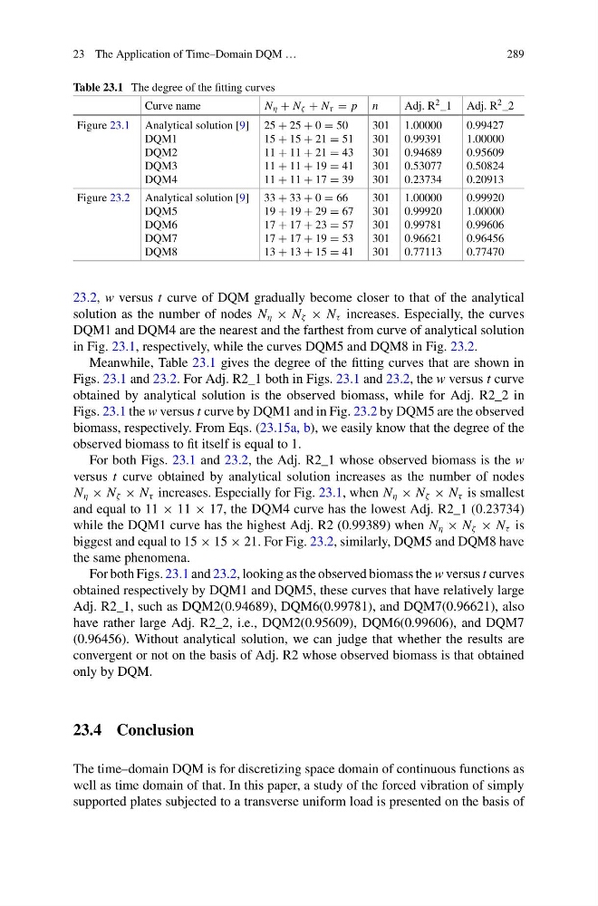
23.2, w versus t curve of DQM gradually become closer to that of the analytical
solution as the number of nodes N η × N ζ × N τ increases. Especially, the curves
DQM1 and DQM4 are the nearest and the farthest from curve of analytical solution
in Fig. 23.1, respectively, while the curves DQM5 and DQM8 in Fig. 23.2.
Meanwhile, Table 23.1 gives the degree of the fitting curves that are shown in
Figs. 23.1 and 23.2. For Adj. R2_1 both in Figs. 23.1 and 23.2, the w versus t curve
obtained by analytical solution is the observed biomass, while for Adj. R2_2 in
Figs. 23.1 the w versus t curve by DQM1 and in Fig. 23.2 by DQM5 are the observed
biomass, respectively. From Eqs. (23.15a, b), we easily know that the degree of the
observed biomass to fit itself is equal to 1.
For both Figs. 23.1 and 23.2, the Adj. R2_1 whose observed biomass is the w
versus t curve obtained by analytical solution increases as the number of nodes
N η × N ζ × N τ increases. Especially for Fig. 23.1, when N η × N ζ × N τ is smallest
and equal to 11 × 11 × 17, the DQM4 curve has the lowest Adj. R2_1 (0.23734)
while the DQM1 curve has the highest Adj. R2 (0.99389) when N η × N ζ × N τ is
biggest and equal to 15 × 15 × 21. For Fig. 23.2, similarly, DQM5 and DQM8 have
the same phenomena.
For both Figs. 23.1 and 23.2, looking as the observed biomass the w versus t curves
obtained respectively by DQM1 and DQM5, these curves that have relatively large
Adj. R2_1, such as DQM2(0.94689), DQM6(0.99781), and DQM7(0.96621), also
have rather large Adj. R2_2, i.e., DQM2(0.95609), DQM6(0.99606), and DQM7
(0.96456). Without analytical solution, we can judge that whether the results are
convergent or not on the basis of Adj. R2 whose observed biomass is that obtained
only by DQM.
23.4 Conclusion
The time–domain DQM is for discretizing space domain of continuous functions as
well as time domain of that. In this paper, a study of the forced vibration of simply
supported plates subjected to a transverse uniform load is presented on the basis of
289
Table 23.1 The degree of the fitting curves
Curve name
N η + N ζ + N τ = p n
Adj. R 2 _1 Adj. R 2 _2
Figure 23.1 Analytical solution [9]
DQM1
DQM2
DQM3
DQM4
25 + 25 + 0 = 50
15 + 15 + 21 = 51
11 + 11 + 21 = 43
11 + 11 + 19 = 41
11 + 11 + 17 = 39
301
301
301
301
301
1.00000
0.99391
0.94689
0.53077
0.23734
0.99427
1.00000
0.95609
0.50824
0.20913
Figure 23.2 Analytical solution [9]
DQM5
DQM6
DQM7
DQM8
33 + 33 + 0 = 66
19 + 19 + 29 = 67
17 + 17 + 23 = 57
17 + 17 + 19 = 53
13 + 13 + 15 = 41
301
301
301
301
301
1.00000
0.99920
0.99781
0.96621
0.77113
0.99920
1.00000
0.99606
0.96456
0.77470
23.2, w versus t curve of DQM gradually become closer to that of the analytical
solution as the number of nodes N η × N ζ × N τ increases. Especially, the curves
DQM1 and DQM4 are the nearest and the farthest from curve of analytical solution
in Fig. 23.1, respectively, while the curves DQM5 and DQM8 in Fig. 23.2.
Meanwhile, Table 23.1 gives the degree of the fitting curves that are shown in
Figs. 23.1 and 23.2. For Adj. R2_1 both in Figs. 23.1 and 23.2, the w versus t curve
obtained by analytical solution is the observed biomass, while for Adj. R2_2 in
Figs. 23.1 the w versus t curve by DQM1 and in Fig. 23.2 by DQM5 are the observed
biomass, respectively. From Eqs. (23.15a, b), we easily know that the degree of the
observed biomass to fit itself is equal to 1.
For both Figs. 23.1 and 23.2, the Adj. R2_1 whose observed biomass is the w
versus t curve obtained by analytical solution increases as the number of nodes
N η × N ζ × N τ increases. Especially for Fig. 23.1, when N η × N ζ × N τ is smallest
and equal to 11 × 11 × 17, the DQM4 curve has the lowest Adj. R2_1 (0.23734)
while the DQM1 curve has the highest Adj. R2 (0.99389) when N η × N ζ × N τ is
biggest and equal to 15 × 15 × 21. For Fig. 23.2, similarly, DQM5 and DQM8 have
the same phenomena.
For both Figs. 23.1 and 23.2, looking as the observed biomass the w versus t curves
obtained respectively by DQM1 and DQM5, these curves that have relatively large
Adj. R2_1, such as DQM2(0.94689), DQM6(0.99781), and DQM7(0.96621), also
have rather large Adj. R2_2, i.e., DQM2(0.95609), DQM6(0.99606), and DQM7
(0.96456). Without analytical solution, we can judge that whether the results are
convergent or not on the basis of Adj. R2 whose observed biomass is that obtained
only by DQM.
23.4 Conclusion
The time–domain DQM is for discretizing space domain of continuous functions as
well as time domain of that. In this paper, a study of the forced vibration of simply
supported plates subjected to a transverse uniform load is presented on the basis of