

288
F. Lin et al.
Eqs. (23.15a, b) [11].
Ad j.R
2
= 1 −
n − 1
n − p
(1 − R
2
), R
2
= 1 −
n
i=1
(w
i
− ˆ
w
i
)
2
/
n
i=1
(w
i
− ¯
w)
2
(23.15a, b)
in which w
i are values of the analytical solution of w at t i = (i − 1)Γ /(n − 1), ˆ
w
i
are that of the DQM, ¯
w is the average value of w
i , n is the sample size of w
i , for
examples, n = 301 in this paper, p is the number of parameters, namely N η + N ζ + N τ ,
and Γ is a period of vibration time t.
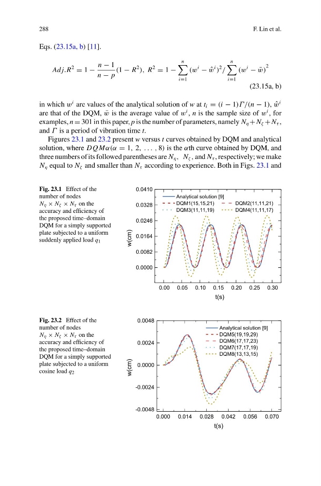
Figures 23.1 and 23.2 present w versus t curves obtained by DQM and analytical
solution, where D Q Mα(α = 1, 2, . . . , 8) is the αth curve obtained by DQM, and
three numbers of its followed parentheses are N η , N ζ , and N τ , respectively; we make
N η equal to N ζ and smaller than N τ according to experience. Both in Figs. 23.1 and
Fig. 23.1 Effect of the
number of nodes
N η × N ζ × N τ on the
accuracy and efficiency of
the proposed time–domain
DQM for a simply supported
plate subjected to a uniform
suddenly applied load q 1
0.00 0.05 0.10 0.15 0.20 0.25 0.30
0.0000
0.0082
0.0164
0.0246
0.0328
0.0410
t(s)
w(cm)
Analytical solution [9]
DQM1(15,15,21)
DQM2(11,11,21)
DQM3(11,11,19)
DQM4(11,11,17)
Fig. 23.2 Effect of the
number of nodes
N η × N ζ × N τ on the
accuracy and efficiency of
the proposed time–domain
DQM for a simply supported
plate subjected to a uniform
cosine load q 2
0.000 0.014 0.028 0.042 0.056 0.070
-0.0048
-0.0024
0.0000
0.0024
0.0048
w(cm)
t(s)
Analytical solution [9]
DQM5(19,19,29)
DQM6(17,17,23)
DQM7(17,17,19)
DQM8(13,13,15)
F. Lin et al.
Eqs. (23.15a, b) [11].
Ad j.R
2
= 1 −
n − 1
n − p
(1 − R
2
), R
2
= 1 −
n
i=1
(w
i
− ˆ
w
i
)
2
/
n
i=1
(w
i
− ¯
w)
2
(23.15a, b)
in which w
i are values of the analytical solution of w at t i = (i − 1)Γ /(n − 1), ˆ
w
i
are that of the DQM, ¯
w is the average value of w
i , n is the sample size of w
i , for
examples, n = 301 in this paper, p is the number of parameters, namely N η + N ζ + N τ ,
and Γ is a period of vibration time t.
Figures 23.1 and 23.2 present w versus t curves obtained by DQM and analytical
solution, where D Q Mα(α = 1, 2, . . . , 8) is the αth curve obtained by DQM, and
three numbers of its followed parentheses are N η , N ζ , and N τ , respectively; we make
N η equal to N ζ and smaller than N τ according to experience. Both in Figs. 23.1 and
Fig. 23.1 Effect of the
number of nodes
N η × N ζ × N τ on the
accuracy and efficiency of
the proposed time–domain
DQM for a simply supported
plate subjected to a uniform
suddenly applied load q 1
0.00 0.05 0.10 0.15 0.20 0.25 0.30
0.0000
0.0082
0.0164
0.0246
0.0328
0.0410
t(s)
w(cm)
Analytical solution [9]
DQM1(15,15,21)
DQM2(11,11,21)
DQM3(11,11,19)
DQM4(11,11,17)
Fig. 23.2 Effect of the
number of nodes
N η × N ζ × N τ on the
accuracy and efficiency of
the proposed time–domain
DQM for a simply supported
plate subjected to a uniform
cosine load q 2
0.000 0.014 0.028 0.042 0.056 0.070
-0.0048
-0.0024
0.0000
0.0024
0.0048
w(cm)
t(s)
Analytical solution [9]
DQM5(19,19,29)
DQM6(17,17,23)
DQM7(17,17,19)
DQM8(13,13,15)