

23 The Application of Time–Domain DQM …
285
w = 0,
∂
2
w
∂ x 2 = 0 at x = 0 and L; w = 0,
∂
2
w
∂ y 2 = 0, y = 0 and B (23.3a–d)
where L and B are length and width, respectively.
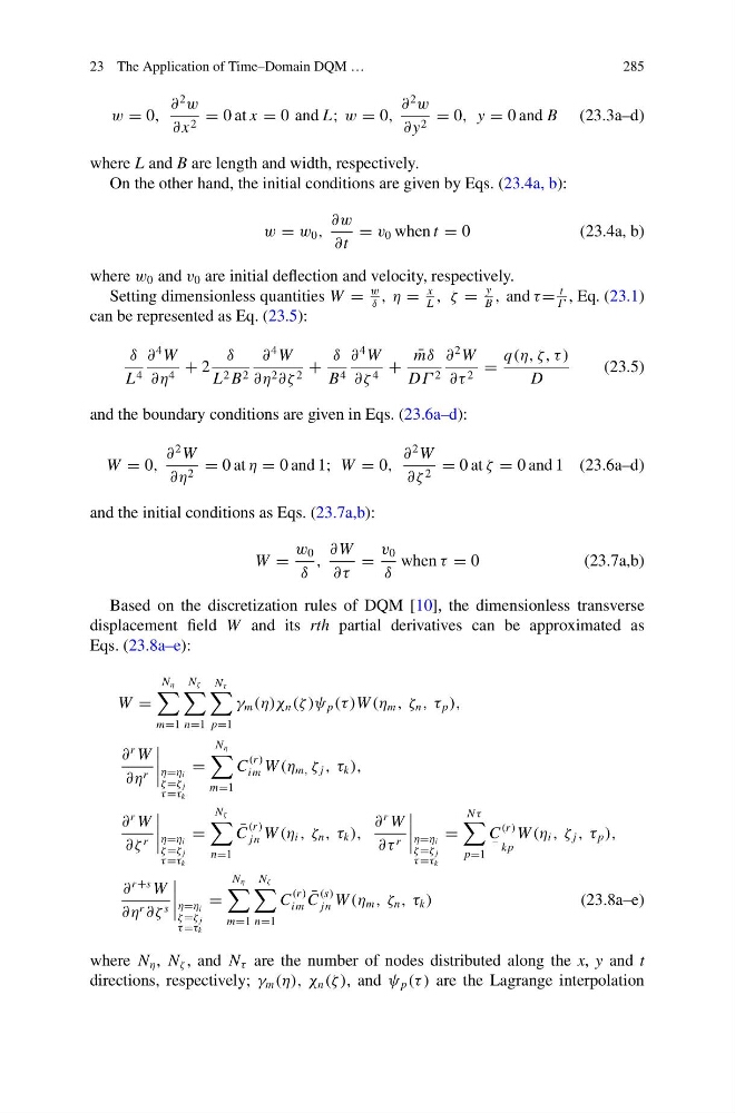
On the other hand, the initial conditions are given by Eqs. (23.4a, b):
w = w 0 ,
∂w
∂t
= v 0 when t = 0
(23.4a, b)
where w 0 and v 0 are initial deflection and velocity, respectively.
Setting dimensionless quantities W =
w
δ
, η =
x
L
, ζ =
y
B
, and τ =
t
Γ
, Eq. (23.1)
can be represented as Eq. (23.5):
δ
L 4
∂
4 W
∂η 4 + 2
δ
L 2 B 2
∂
4 W
∂η 2 ∂ζ 2 +
δ
B 4
∂
4 W
∂ζ 4 +
¯
mδ
DΓ 2
∂
2 W
∂τ 2 =
q(η, ζ, τ )
D
(23.5)
and the boundary conditions are given in Eqs. (23.6a–d):
W = 0,
∂
2 W
∂η 2 = 0 at η = 0 and 1; W = 0,
∂
2 W
∂ζ 2 = 0 at ζ = 0 and 1 (23.6a–d)
and the initial conditions as Eqs. (23.7a,b):
W =
w 0
δ
,
∂ W
∂τ
=
v 0
δ
when τ = 0
(23.7a,b)
Based on the discretization rules of DQM [10], the dimensionless transverse
displacement field W and its rth partial derivatives can be approximated as
Eqs. (23.8a–e):
W =
N η
m=1
N ζ
n=1
N τ
p=1
γ m (η)χ n (ζ )ψ p (τ )W (η m , ζ n , τ p ),
∂
r W
∂η r
η=ηi
ζ =ζ j
τ =τ k
=
N η
m=1
C
(r )
im W (η m, ζ j , τ k ),
∂
r W
∂ζ r
η=ηi
ζ =ζ j
τ =τ k
=
N ζ
n=1
¯
C
(r )
jn W (η i , ζ n , τ k ),
∂
r W
∂τ r
η=ηi
ζ =ζ j
τ =τ k
=
N τ
p=1
C −
(r )
kp
W (η i , ζ j , τ p ),
∂
r +s W
∂η r ∂ζ s
η=ηi
ζ =ζ j
τ =τ k
=
N η
m=1
N ζ
n=1
C
(r )
im
¯
C
(s)
jn W (η m , ζ n , τ k )
(23.8a–e)
where N η , N ζ , and N τ are the number of nodes distributed along the x, y and t
directions, respectively; γ m (η), χ n (ζ ), and ψ p (τ ) are the Lagrange interpolation
285
w = 0,
∂
2
w
∂ x 2 = 0 at x = 0 and L; w = 0,
∂
2
w
∂ y 2 = 0, y = 0 and B (23.3a–d)
where L and B are length and width, respectively.
On the other hand, the initial conditions are given by Eqs. (23.4a, b):
w = w 0 ,
∂w
∂t
= v 0 when t = 0
(23.4a, b)
where w 0 and v 0 are initial deflection and velocity, respectively.
Setting dimensionless quantities W =
w
δ
, η =
x
L
, ζ =
y
B
, and τ =
t
Γ
, Eq. (23.1)
can be represented as Eq. (23.5):
δ
L 4
∂
4 W
∂η 4 + 2
δ
L 2 B 2
∂
4 W
∂η 2 ∂ζ 2 +
δ
B 4
∂
4 W
∂ζ 4 +
¯
mδ
DΓ 2
∂
2 W
∂τ 2 =
q(η, ζ, τ )
D
(23.5)
and the boundary conditions are given in Eqs. (23.6a–d):
W = 0,
∂
2 W
∂η 2 = 0 at η = 0 and 1; W = 0,
∂
2 W
∂ζ 2 = 0 at ζ = 0 and 1 (23.6a–d)
and the initial conditions as Eqs. (23.7a,b):
W =
w 0
δ
,
∂ W
∂τ
=
v 0
δ
when τ = 0
(23.7a,b)
Based on the discretization rules of DQM [10], the dimensionless transverse
displacement field W and its rth partial derivatives can be approximated as
Eqs. (23.8a–e):
W =
N η
m=1
N ζ
n=1
N τ
p=1
γ m (η)χ n (ζ )ψ p (τ )W (η m , ζ n , τ p ),
∂
r W
∂η r
η=ηi
ζ =ζ j
τ =τ k
=
N η
m=1
C
(r )
im W (η m, ζ j , τ k ),
∂
r W
∂ζ r
η=ηi
ζ =ζ j
τ =τ k
=
N ζ
n=1
¯
C
(r )
jn W (η i , ζ n , τ k ),
∂
r W
∂τ r
η=ηi
ζ =ζ j
τ =τ k
=
N τ
p=1
C −
(r )
kp
W (η i , ζ j , τ p ),
∂
r +s W
∂η r ∂ζ s
η=ηi
ζ =ζ j
τ =τ k
=
N η
m=1
N ζ
n=1
C
(r )
im
¯
C
(s)
jn W (η m , ζ n , τ k )
(23.8a–e)
where N η , N ζ , and N τ are the number of nodes distributed along the x, y and t
directions, respectively; γ m (η), χ n (ζ ), and ψ p (τ ) are the Lagrange interpolation