

1 Controlled and Localized Electrochemical Microfabrication …
7
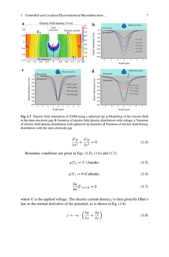
Fig. 1.3 Electric field simulation of EMM using a spherical tip, a Modelling of the electric field
in the inter-electrode gap, b Variation of electric field density distribution with voltage, c Variation
of electric field density distribution with spherical tip diameter, d Variation of electric field density
distribution with the inter-electrode gap
∂
2
ϕ
∂ x 2 +
∂
2
ϕ
∂ y 2 = 0
( 1 . 4 )
Boundary conditions are given in Eqs. (1.5), (1.6) and (1.7):
ϕ| 2 = U (Anode)
(1.5)
ϕ| 1 = 0 (Cathode)
(1.6)
∂ϕ
∂n
| 3,4,5,6 = 0
(1.7)
where U is the applied voltage. The electric current density j is then given by Ohm’s
law as the normal derivative of the potential, as is shown in Eq. (1.8)
j = −κ ·
∂ϕ
∂ x
+
∂ϕ
∂ y
(1.8)
7
Fig. 1.3 Electric field simulation of EMM using a spherical tip, a Modelling of the electric field
in the inter-electrode gap, b Variation of electric field density distribution with voltage, c Variation
of electric field density distribution with spherical tip diameter, d Variation of electric field density
distribution with the inter-electrode gap
∂
2
ϕ
∂ x 2 +
∂
2
ϕ
∂ y 2 = 0
( 1 . 4 )
Boundary conditions are given in Eqs. (1.5), (1.6) and (1.7):
ϕ| 2 = U (Anode)
(1.5)
ϕ| 1 = 0 (Cathode)
(1.6)
∂ϕ
∂n
| 3,4,5,6 = 0
(1.7)
where U is the applied voltage. The electric current density j is then given by Ohm’s
law as the normal derivative of the potential, as is shown in Eq. (1.8)
j = −κ ·
∂ϕ
∂ x
+
∂ϕ
∂ y
(1.8)