

126
Y. Ge and Z. Ye
variance retained for different values decides the number of components that retained
by Eq. (10.10):
k
i=1 λ i
n
i=1 λ i
(10.10)
where λ 1 , . . . , λ k are the eigenvalues of the covariance matrix of the dataset. As
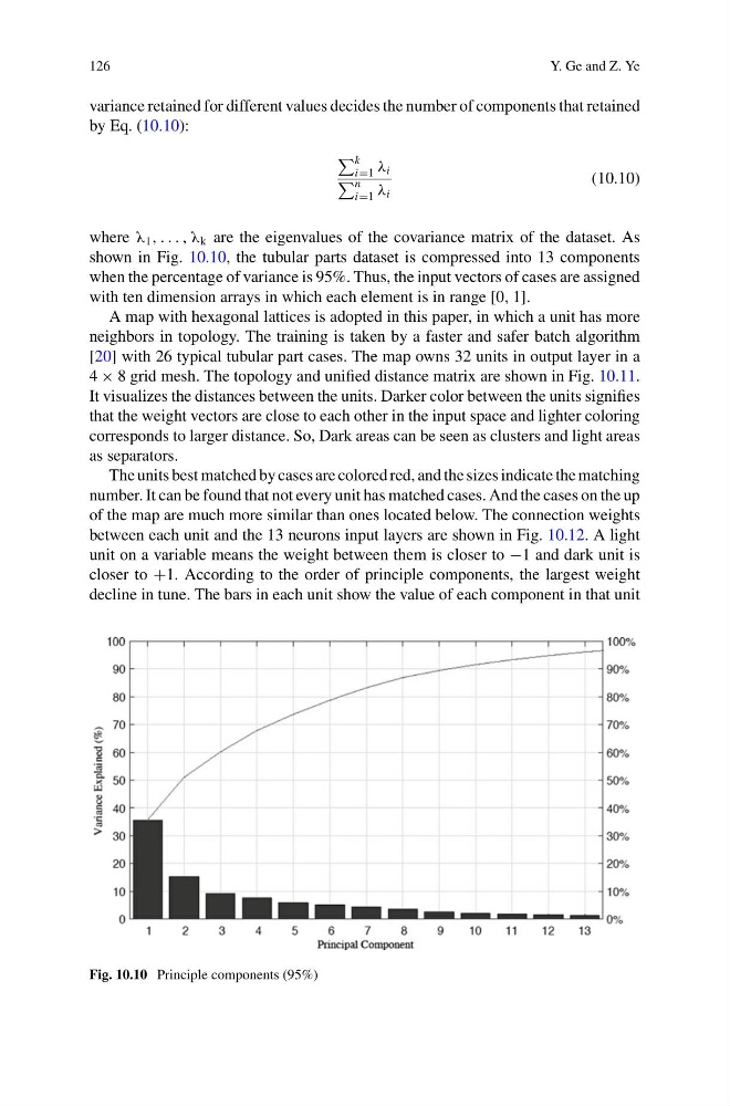
shown in Fig. 10.10, the tubular parts dataset is compressed into 13 components
when the percentage of variance is 95%. Thus, the input vectors of cases are assigned
with ten dimension arrays in which each element is in range [0, 1].
A map with hexagonal lattices is adopted in this paper, in which a unit has more
neighbors in topology. The training is taken by a faster and safer batch algorithm
[20] with 26 typical tubular part cases. The map owns 32 units in output layer in a
4 × 8 grid mesh. The topology and unified distance matrix are shown in Fig. 10.11.
It visualizes the distances between the units. Darker color between the units signifies
that the weight vectors are close to each other in the input space and lighter coloring
corresponds to larger distance. So, Dark areas can be seen as clusters and light areas
as separators.
The units best matched by cases are colored red, and the sizes indicate the matching
number. It can be found that not every unit has matched cases. And the cases on the up
of the map are much more similar than ones located below. The connection weights
between each unit and the 13 neurons input layers are shown in Fig. 10.12. A light
unit on a variable means the weight between them is closer to −1 and dark unit is
closer to +1. According to the order of principle components, the largest weight
decline in tune. The bars in each unit show the value of each component in that unit
Fig. 10.10 Principle components (95%)
Y. Ge and Z. Ye
variance retained for different values decides the number of components that retained
by Eq. (10.10):
k
i=1 λ i
n
i=1 λ i
(10.10)
where λ 1 , . . . , λ k are the eigenvalues of the covariance matrix of the dataset. As
shown in Fig. 10.10, the tubular parts dataset is compressed into 13 components
when the percentage of variance is 95%. Thus, the input vectors of cases are assigned
with ten dimension arrays in which each element is in range [0, 1].
A map with hexagonal lattices is adopted in this paper, in which a unit has more
neighbors in topology. The training is taken by a faster and safer batch algorithm
[20] with 26 typical tubular part cases. The map owns 32 units in output layer in a
4 × 8 grid mesh. The topology and unified distance matrix are shown in Fig. 10.11.
It visualizes the distances between the units. Darker color between the units signifies
that the weight vectors are close to each other in the input space and lighter coloring
corresponds to larger distance. So, Dark areas can be seen as clusters and light areas
as separators.
The units best matched by cases are colored red, and the sizes indicate the matching
number. It can be found that not every unit has matched cases. And the cases on the up
of the map are much more similar than ones located below. The connection weights
between each unit and the 13 neurons input layers are shown in Fig. 10.12. A light
unit on a variable means the weight between them is closer to −1 and dark unit is
closer to +1. According to the order of principle components, the largest weight
decline in tune. The bars in each unit show the value of each component in that unit
Fig. 10.10 Principle components (95%)