

60
6 Nonlocal Gravity
1. < 0, r 1 > 0, r 2 > 0—cyclic Universe (in particular one can have cyclic
inflation).
2. > 0, r 1 < 0, r 2 > 0—first contraction, then very rapid inflation (superinflation) a(t) ∝ exp(kt
2
).
3. > 0, r 1 > 0, r 2 < 0—constant curvature R = 4
M
2
P
, i.e. de Sitter solution.
So we find that accelerating solutions are possible within all these scenarios.
Again, we note that in the constant scalar curvature case, we have drastic reducing
of equations.
Moreover, it has been shown in [117] that for L =
√ |g|
√
R − 2F()
√
R − 2,
with F() being an arbitrary analytic function, there are hyper-exponentially accelerating cosmological solutions a(t) ∝ e
kt
2 .
The next step in study of nonlocal theories consists in introducing non-analytic
functions of the d’Alembertian operator. The simplest case is F() =
1
. Actually it
means that we must consider terms like R
−1 R. It is clear that the gravity extension
with such a term is non-renormalizable since the propagator behaves as only
1
k 2 , so we
gain nothing in comparison with the usual Einstein-Hlbert gravity [118]. However,
theories with negative degrees of the d’Alembertian operator can display new treelevel effects, especially within the cosmological context where an important class
of nonlocal gravity models has been introduced in [119]. The action of this class of
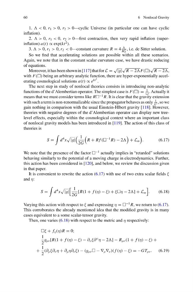
theories is
S =
d
4 x
|g|
1
2G
R + R f (
−1 R) − 2
+ L m
.
(6.17)
We note that the presence of the factor
−1 actually implies in “retarded” solutions
behaving similarly to the potential of a moving charge in electrodynamics. Further,
this action has been considered in [120], and below, we review the discussion given
in that paper.
It is convenient to rewrite the action (6.17) with use of two extra scalar fields ξ
and η:
S =
d
4 x
|g|
1
2G
[R(1 + f (η) − ξ) + ξη − 2] + L m
.
(6.18)
Varying this action with respect to ξ and expressing η =
−1 R, we return to (6.17).
This corroborates the already mentioned idea that the modified gravity is in many
cases equivalent to a some scalar-tensor gravity.
Then, one varies (6.18) with respect to the metric and η respectively:
ξ + f η (η)R = 0;
1
2
g μν [R(1 + f (η) − ξ) − ∂ α ξ∂
α
η − 2] − R μν (1 + f (η) − ξ) +
+
1
2
(∂ μ ξ∂ ν η + ∂ μ η∂ ν ξ) − (g μν − ∇ μ ∇ ν )( f (η) − ξ) = −GT μν .
(6.19)
6 Nonlocal Gravity
1. < 0, r 1 > 0, r 2 > 0—cyclic Universe (in particular one can have cyclic
inflation).
2. > 0, r 1 < 0, r 2 > 0—first contraction, then very rapid inflation (superinflation) a(t) ∝ exp(kt
2
).
3. > 0, r 1 > 0, r 2 < 0—constant curvature R = 4
M
2
P
, i.e. de Sitter solution.
So we find that accelerating solutions are possible within all these scenarios.
Again, we note that in the constant scalar curvature case, we have drastic reducing
of equations.
Moreover, it has been shown in [117] that for L =
√ |g|
√
R − 2F()
√
R − 2,
with F() being an arbitrary analytic function, there are hyper-exponentially accelerating cosmological solutions a(t) ∝ e
kt
2 .
The next step in study of nonlocal theories consists in introducing non-analytic
functions of the d’Alembertian operator. The simplest case is F() =
1
. Actually it
means that we must consider terms like R
−1 R. It is clear that the gravity extension
with such a term is non-renormalizable since the propagator behaves as only
1
k 2 , so we
gain nothing in comparison with the usual Einstein-Hlbert gravity [118]. However,
theories with negative degrees of the d’Alembertian operator can display new treelevel effects, especially within the cosmological context where an important class
of nonlocal gravity models has been introduced in [119]. The action of this class of
theories is
S =
d
4 x
|g|
1
2G
R + R f (
−1 R) − 2
+ L m
.
(6.17)
We note that the presence of the factor
−1 actually implies in “retarded” solutions
behaving similarly to the potential of a moving charge in electrodynamics. Further,
this action has been considered in [120], and below, we review the discussion given
in that paper.
It is convenient to rewrite the action (6.17) with use of two extra scalar fields ξ
and η:
S =
d
4 x
|g|
1
2G
[R(1 + f (η) − ξ) + ξη − 2] + L m
.
(6.18)
Varying this action with respect to ξ and expressing η =
−1 R, we return to (6.17).
This corroborates the already mentioned idea that the modified gravity is in many
cases equivalent to a some scalar-tensor gravity.
Then, one varies (6.18) with respect to the metric and η respectively:
ξ + f η (η)R = 0;
1
2
g μν [R(1 + f (η) − ξ) − ∂ α ξ∂
α
η − 2] − R μν (1 + f (η) − ξ) +
+
1
2
(∂ μ ξ∂ ν η + ∂ μ η∂ ν ξ) − (g μν − ∇ μ ∇ ν )( f (η) − ξ) = −GT μν .
(6.19)