

48
5 Horava–Lifshitz Gravity
In this chapter we present a general review on HL gravity, introduce definitions
of main quantities used within it, and describe most important classical solutions.
5.2 Basic Definitions
So, let us construct the gravity model on the base of a strong difference between time
and space coordinates. Following the methodology developed in [93], we consider
the space-time as a foliation R × M 3 , where R is the real axis corresponding to the
time, and M 3 is the three-dimensional manifold parametrized by spatial coordinates.
The most convenient variables to parametrize the gravitational field in this case are
the Arnowitt–Deser–Misner (ADM) variables [95], that is, N , N i , g i j defined from
the following representation of the metric:
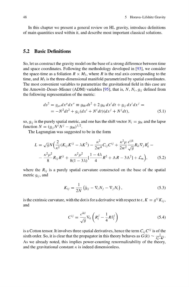
ds
2
= g μν dx
μ dx
ν
≡ g 00 dt
2
+ 2 g 0i dx
i dt + g i j dx
i dx
j
=
= −N
2 dt
2
+ g i j (dx
i
+ N
i dt)(dx
j
+ N
j dt),
(5.1)
so, g i j is the purely spatial metric, and one has the shift vector N i = g 0i and the lapse
function N = (g i j N
i N
j
− g 00 )
1/2 .
The Lagrangian was suggested to be in the form
L =
√ g N
2
κ 2 (K i j K
i j
− λK
2
) −
κ
2
2w 4 C i j C
i j
+
κ
2
μ
2w 2
i jk
√
g
R il ∇ j R
l
k −
−
κ
2
μ
2
8
R i j R
i j
+
κ
2
μ
2
8(1 − 3λ)
[
1 − 4λ
4
R
2
+ R − 3
2
] + L m
,
(5.2)
where the R i j is a purely spatial curvature constructed on the base of the spatial
metric g i j , and
K i j =
1
2N
˙
g i j − ∇ i N j − ∇ j N i
,
(5.3)
is the extrinsic curvature, with the dot is for a derivative with respect to t, K = g
i j K i j ,
and
C
i j
=
ikl
√ g
∇ k
R
j
l −
1
4
Rδ
j
l
(5.4)
is a Cotton tensor. It involves three spatial derivatives, hence the term C i j C
i j is of the
sixth order. So, it is clear that the propagator in this theory behaves as G(k) ∼
1
k
2
0 −k 6 .
As we already noted, this implies power-counting renormalizability of the theory,
and the gravitational constant κ is indeed dimensionless.
5 Horava–Lifshitz Gravity
In this chapter we present a general review on HL gravity, introduce definitions
of main quantities used within it, and describe most important classical solutions.
5.2 Basic Definitions
So, let us construct the gravity model on the base of a strong difference between time
and space coordinates. Following the methodology developed in [93], we consider
the space-time as a foliation R × M 3 , where R is the real axis corresponding to the
time, and M 3 is the three-dimensional manifold parametrized by spatial coordinates.
The most convenient variables to parametrize the gravitational field in this case are
the Arnowitt–Deser–Misner (ADM) variables [95], that is, N , N i , g i j defined from
the following representation of the metric:
ds
2
= g μν dx
μ dx
ν
≡ g 00 dt
2
+ 2 g 0i dx
i dt + g i j dx
i dx
j
=
= −N
2 dt
2
+ g i j (dx
i
+ N
i dt)(dx
j
+ N
j dt),
(5.1)
so, g i j is the purely spatial metric, and one has the shift vector N i = g 0i and the lapse
function N = (g i j N
i N
j
− g 00 )
1/2 .
The Lagrangian was suggested to be in the form
L =
√ g N
2
κ 2 (K i j K
i j
− λK
2
) −
κ
2
2w 4 C i j C
i j
+
κ
2
μ
2w 2
i jk
√
g
R il ∇ j R
l
k −
−
κ
2
μ
2
8
R i j R
i j
+
κ
2
μ
2
8(1 − 3λ)
[
1 − 4λ
4
R
2
+ R − 3
2
] + L m
,
(5.2)
where the R i j is a purely spatial curvature constructed on the base of the spatial
metric g i j , and
K i j =
1
2N
˙
g i j − ∇ i N j − ∇ j N i
,
(5.3)
is the extrinsic curvature, with the dot is for a derivative with respect to t, K = g
i j K i j ,
and
C
i j
=
ikl
√ g
∇ k
R
j
l −
1
4
Rδ
j
l
(5.4)
is a Cotton tensor. It involves three spatial derivatives, hence the term C i j C
i j is of the
sixth order. So, it is clear that the propagator in this theory behaves as G(k) ∼
1
k
2
0 −k 6 .
As we already noted, this implies power-counting renormalizability of the theory,
and the gravitational constant κ is indeed dimensionless.