

2.3 f (R)-Gravity
13
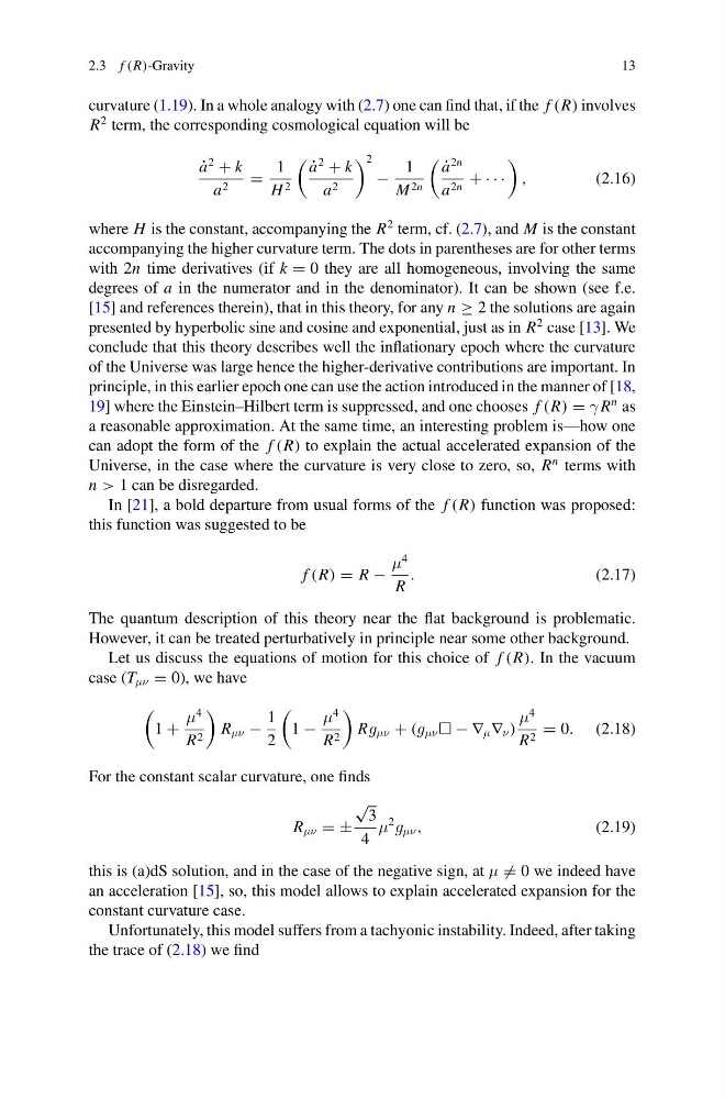
curvature (1.19). In a whole analogy with (2.7) one can find that, if the f (R) involves
R
2 term, the corresponding cosmological equation will be
˙
a
2
+ k
a 2 =
1
H 2
˙
a
2
+ k
a 2
2
−
1
M 2n
˙
a
2n
a 2n + · · ·
,
(2.16)
where H is the constant, accompanying the R
2 term, cf. (2.7), and M is the constant
accompanying the higher curvature term. The dots in parentheses are for other terms
with 2n time derivatives (if k = 0 they are all homogeneous, involving the same
degrees of a in the numerator and in the denominator). It can be shown (see f.e.
[15] and references therein), that in this theory, for any n ≥ 2 the solutions are again
presented by hyperbolic sine and cosine and exponential, just as in R
2 case [13]. We
conclude that this theory describes well the inflationary epoch where the curvature
of the Universe was large hence the higher-derivative contributions are important. In
principle, in this earlier epoch one can use the action introduced in the manner of [18,
19] where the Einstein–Hilbert term is suppressed, and one chooses f (R) = γ R
n as
a reasonable approximation. At the same time, an interesting problem is—how one
can adopt the form of the f (R) to explain the actual accelerated expansion of the
Universe, in the case where the curvature is very close to zero, so, R
n terms with
n > 1 can be disregarded.
In [21], a bold departure from usual forms of the f (R) function was proposed:
this function was suggested to be
f (R) = R −
μ
4
R
.
(2.17)
The quantum description of this theory near the flat background is problematic.
However, it can be treated perturbatively in principle near some other background.
Let us discuss the equations of motion for this choice of f (R). In the vacuum
case (T μν = 0), we have
1 +
μ
4
R 2
R μν −
1
2
1 −
μ
4
R 2
Rg μν + (g μν − ∇ μ ∇ ν )
μ
4
R 2 = 0. (2.18)
For the constant scalar curvature, one finds
R μν = ±
√
3
4
μ
2
g μν ,
(2.19)
this is (a)dS solution, and in the case of the negative sign, at μ = 0 we indeed have
an acceleration [15], so, this model allows to explain accelerated expansion for the
constant curvature case.
Unfortunately, this model suffers from a tachyonic instability. Indeed, after taking
the trace of (2.18) we find
13
curvature (1.19). In a whole analogy with (2.7) one can find that, if the f (R) involves
R
2 term, the corresponding cosmological equation will be
˙
a
2
+ k
a 2 =
1
H 2
˙
a
2
+ k
a 2
2
−
1
M 2n
˙
a
2n
a 2n + · · ·
,
(2.16)
where H is the constant, accompanying the R
2 term, cf. (2.7), and M is the constant
accompanying the higher curvature term. The dots in parentheses are for other terms
with 2n time derivatives (if k = 0 they are all homogeneous, involving the same
degrees of a in the numerator and in the denominator). It can be shown (see f.e.
[15] and references therein), that in this theory, for any n ≥ 2 the solutions are again
presented by hyperbolic sine and cosine and exponential, just as in R
2 case [13]. We
conclude that this theory describes well the inflationary epoch where the curvature
of the Universe was large hence the higher-derivative contributions are important. In
principle, in this earlier epoch one can use the action introduced in the manner of [18,
19] where the Einstein–Hilbert term is suppressed, and one chooses f (R) = γ R
n as
a reasonable approximation. At the same time, an interesting problem is—how one
can adopt the form of the f (R) to explain the actual accelerated expansion of the
Universe, in the case where the curvature is very close to zero, so, R
n terms with
n > 1 can be disregarded.
In [21], a bold departure from usual forms of the f (R) function was proposed:
this function was suggested to be
f (R) = R −
μ
4
R
.
(2.17)
The quantum description of this theory near the flat background is problematic.
However, it can be treated perturbatively in principle near some other background.
Let us discuss the equations of motion for this choice of f (R). In the vacuum
case (T μν = 0), we have
1 +
μ
4
R 2
R μν −
1
2
1 −
μ
4
R 2
Rg μν + (g μν − ∇ μ ∇ ν )
μ
4
R 2 = 0. (2.18)
For the constant scalar curvature, one finds
R μν = ±
√
3
4
μ
2
g μν ,
(2.19)
this is (a)dS solution, and in the case of the negative sign, at μ = 0 we indeed have
an acceleration [15], so, this model allows to explain accelerated expansion for the
constant curvature case.
Unfortunately, this model suffers from a tachyonic instability. Indeed, after taking
the trace of (2.18) we find