

40
2 Description of the Wolfram SystemModeler
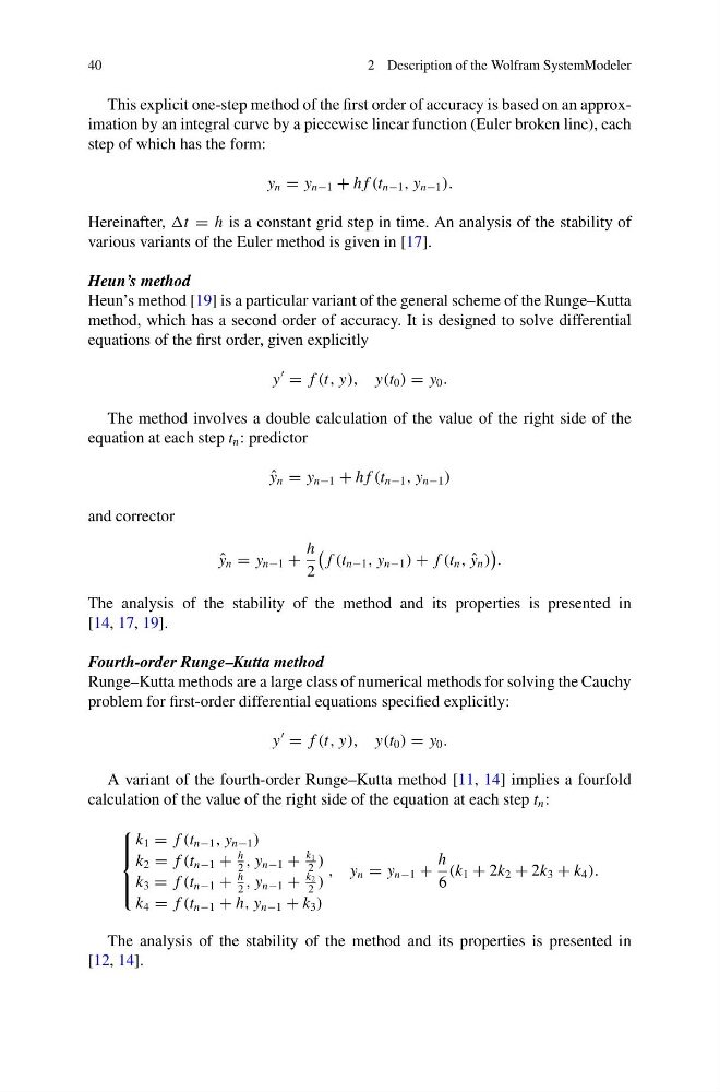
This explicit one-step method of the first order of accuracy is based on an approximation by an integral curve by a piecewise linear function (Euler broken line), each
step of which has the form:
y n = y n−1 + h f (t n−1 , y n−1 ).
Hereinafter, t = h is a constant grid step in time. An analysis of the stability of
various variants of the Euler method is given in [17].
Heun’s method
Heun’s method [19] is a particular variant of the general scheme of the Runge–Kutta
method, which has a second order of accuracy. It is designed to solve differential
equations of the first order, given explicitly
y
= f (t, y), y(t 0 ) = y 0 .
The method involves a double calculation of the value of the right side of the
equation at each step t n : predictor
ˆ
y n = y n−1 + h f (t n−1 , y n−1 )
and corrector
ˆ
y n = y n−1 +
h
2
f (t n−1 , y n−1 ) + f (t n , ˆ
y n )
.
The analysis of the stability of the method and its properties is presented in
[14, 17, 19].
Fourth-order Runge–Kutta method
Runge–Kutta methods are a large class of numerical methods for solving the Cauchy
problem for first-order differential equations specified explicitly:
y
= f (t, y), y(t 0 ) = y 0 .
A variant of the fourth-order Runge–Kutta method [11, 14] implies a fourfold
calculation of the value of the right side of the equation at each step t n :
⎧
⎪ ⎪ ⎨
⎪ ⎪ ⎩
k 1 = f (t n−1 , y n−1 )
k 2 = f (t n−1 +
h
2
, y n−1 +
k 1
2
)
k 3 = f (t n−1 +
h
2
, y n−1 +
k 2
2
)
k 4 = f (t n−1 + h, y n−1 + k 3 )
, y n = y n−1 +
h
6
(k 1 + 2k 2 + 2k 3 + k 4 ).
The analysis of the stability of the method and its properties is presented in
[12, 14].
2 Description of the Wolfram SystemModeler
This explicit one-step method of the first order of accuracy is based on an approximation by an integral curve by a piecewise linear function (Euler broken line), each
step of which has the form:
y n = y n−1 + h f (t n−1 , y n−1 ).
Hereinafter, t = h is a constant grid step in time. An analysis of the stability of
various variants of the Euler method is given in [17].
Heun’s method
Heun’s method [19] is a particular variant of the general scheme of the Runge–Kutta
method, which has a second order of accuracy. It is designed to solve differential
equations of the first order, given explicitly
y
= f (t, y), y(t 0 ) = y 0 .
The method involves a double calculation of the value of the right side of the
equation at each step t n : predictor
ˆ
y n = y n−1 + h f (t n−1 , y n−1 )
and corrector
ˆ
y n = y n−1 +
h
2
f (t n−1 , y n−1 ) + f (t n , ˆ
y n )
.
The analysis of the stability of the method and its properties is presented in
[14, 17, 19].
Fourth-order Runge–Kutta method
Runge–Kutta methods are a large class of numerical methods for solving the Cauchy
problem for first-order differential equations specified explicitly:
y
= f (t, y), y(t 0 ) = y 0 .
A variant of the fourth-order Runge–Kutta method [11, 14] implies a fourfold
calculation of the value of the right side of the equation at each step t n :
⎧
⎪ ⎪ ⎨
⎪ ⎪ ⎩
k 1 = f (t n−1 , y n−1 )
k 2 = f (t n−1 +
h
2
, y n−1 +
k 1
2
)
k 3 = f (t n−1 +
h
2
, y n−1 +
k 2
2
)
k 4 = f (t n−1 + h, y n−1 + k 3 )
, y n = y n−1 +
h
6
(k 1 + 2k 2 + 2k 3 + k 4 ).
The analysis of the stability of the method and its properties is presented in
[12, 14].