

214
6 Hierarchical Component Models
Real u(unit = ”m3/s”) ”Output flow demanded by controller”;
Real e(unit = ”m”) ”Deviation from reference level”;
Real x(unit = ”m”) ”State variable for controller”;
equation
assert(minFlow >= 0, ”minFlow - minimum flow through
output valve must be >= 0”);
der(h) = (qIn - qOut) / A;
qIn = if time > 150 then 3 * q0 else q0;
qOutMax = if h > 0 then maxFlow else min(qIn, maxFlow);
qOut = if (-u) < minFlow then minFlow elseif (-u) >
qOutMax then qOutMax else -u;
e = ref - h;
der(x) = e / T;
u = K * (e + x);
end FlatTank;
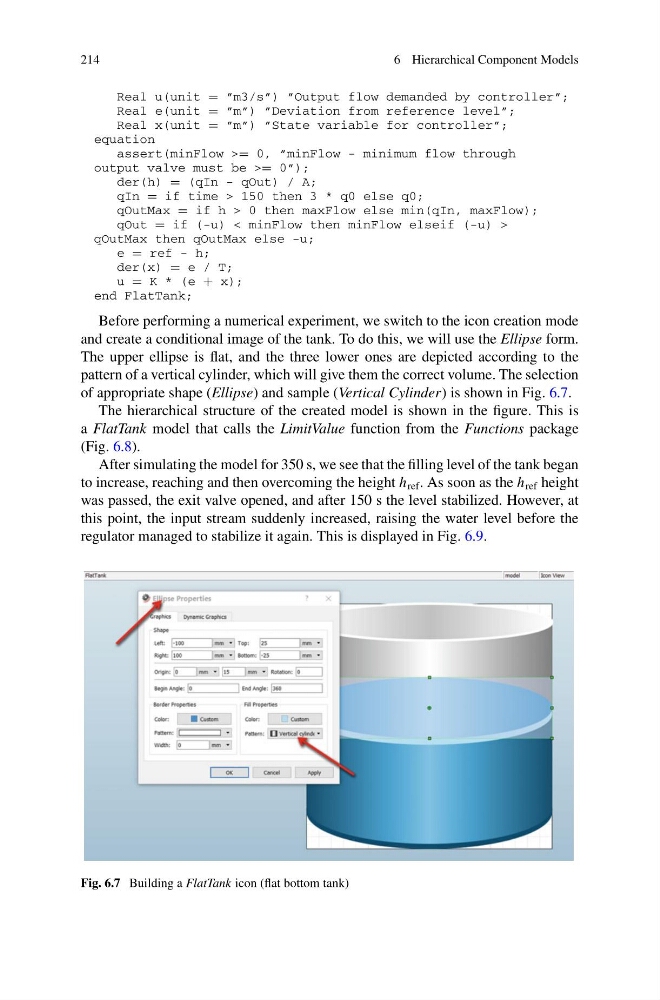
Before performing a numerical experiment, we switch to the icon creation mode
and create a conditional image of the tank. To do this, we will use the Ellipse form.
The upper ellipse is flat, and the three lower ones are depicted according to the
pattern of a vertical cylinder, which will give them the correct volume. The selection
of appropriate shape (Ellipse) and sample (Vertical Cylinder) is shown in Fig. 6.7.
The hierarchical structure of the created model is shown in the figure. This is
a FlatTank model that calls the LimitValue function from the Functions package
(Fig. 6.8).
After simulating the model for 350 s, we see that the filling level of the tank began
to increase, reaching and then overcoming the height h ref . As soon as the h ref height
was passed, the exit valve opened, and after 150 s the level stabilized. However, at
this point, the input stream suddenly increased, raising the water level before the
regulator managed to stabilize it again. This is displayed in Fig. 6.9.
Fig. 6.7 Building a FlatTank icon (flat bottom tank)
6 Hierarchical Component Models
Real u(unit = ”m3/s”) ”Output flow demanded by controller”;
Real e(unit = ”m”) ”Deviation from reference level”;
Real x(unit = ”m”) ”State variable for controller”;
equation
assert(minFlow >= 0, ”minFlow - minimum flow through
output valve must be >= 0”);
der(h) = (qIn - qOut) / A;
qIn = if time > 150 then 3 * q0 else q0;
qOutMax = if h > 0 then maxFlow else min(qIn, maxFlow);
qOut = if (-u) < minFlow then minFlow elseif (-u) >
qOutMax then qOutMax else -u;
e = ref - h;
der(x) = e / T;
u = K * (e + x);
end FlatTank;
Before performing a numerical experiment, we switch to the icon creation mode
and create a conditional image of the tank. To do this, we will use the Ellipse form.
The upper ellipse is flat, and the three lower ones are depicted according to the
pattern of a vertical cylinder, which will give them the correct volume. The selection
of appropriate shape (Ellipse) and sample (Vertical Cylinder) is shown in Fig. 6.7.
The hierarchical structure of the created model is shown in the figure. This is
a FlatTank model that calls the LimitValue function from the Functions package
(Fig. 6.8).
After simulating the model for 350 s, we see that the filling level of the tank began
to increase, reaching and then overcoming the height h ref . As soon as the h ref height
was passed, the exit valve opened, and after 150 s the level stabilized. However, at
this point, the input stream suddenly increased, raising the water level before the
regulator managed to stabilize it again. This is displayed in Fig. 6.9.
Fig. 6.7 Building a FlatTank icon (flat bottom tank)