

166
5 Modeling of Mechanical Oscillatory Systems …
dθ 2
dt
= ω 2
dω 2
dt
=
−g
l 2
sin θ 2 −
kd
2
m 2 l
2
2
(sin θ 2 − sin θ 1 ) cos θ 2
where ω 1 and ω 2 are the corresponding angular velocities. In the particular case
of small deviation angles, this system decomposes into two independent equations
in which the variables are the sum of the angular displacements θ 1 + θ 2 and their
difference θ 1 − θ 2 . Moreover, each of these equations describes oscillations of a
harmonic oscillator with natural frequencies ω
+ and ω
− , respectively.
When considering the “symmetric” system, it is necessary to put l 1 = l 2 , m 1 = m 2
in these equations, when considering the “asymmetric” system for the first pendulum
l 1 = d and for the second pendulum l 2 = d.
We begin the simulation with a special case of the mathematical model constructed
above for the case of a symmetric system, i.e., identical pendulums (l 1 = l 2 , m 1 =
m 2 ).
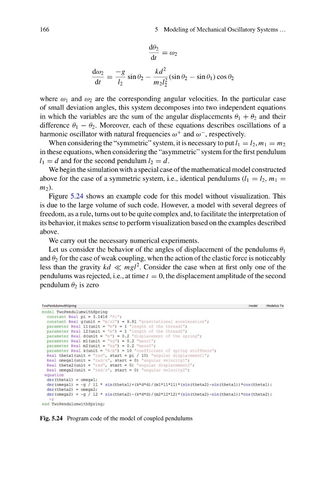
Figure 5.24 shows an example code for this model without visualization. This
is due to the large volume of such code. However, a model with several degrees of
freedom, as a rule, turns out to be quite complex and, to facilitate the interpretation of
its behavior, it makes sense to perform visualization based on the examples described
above.
We carry out the necessary numerical experiments.
Let us consider the behavior of the angles of displacement of the pendulums θ 1
and θ 2 for the case of weak coupling, when the action of the elastic force is noticeably
less than the gravity kd mgl
2 . Consider the case when at first only one of the
pendulums was rejected, i.e., at time t = 0, the displacement amplitude of the second
pendulum θ 2 is zero
Fig. 5.24 Program code of the model of coupled pendulums
5 Modeling of Mechanical Oscillatory Systems …
dθ 2
dt
= ω 2
dω 2
dt
=
−g
l 2
sin θ 2 −
kd
2
m 2 l
2
2
(sin θ 2 − sin θ 1 ) cos θ 2
where ω 1 and ω 2 are the corresponding angular velocities. In the particular case
of small deviation angles, this system decomposes into two independent equations
in which the variables are the sum of the angular displacements θ 1 + θ 2 and their
difference θ 1 − θ 2 . Moreover, each of these equations describes oscillations of a
harmonic oscillator with natural frequencies ω
+ and ω
− , respectively.
When considering the “symmetric” system, it is necessary to put l 1 = l 2 , m 1 = m 2
in these equations, when considering the “asymmetric” system for the first pendulum
l 1 = d and for the second pendulum l 2 = d.
We begin the simulation with a special case of the mathematical model constructed
above for the case of a symmetric system, i.e., identical pendulums (l 1 = l 2 , m 1 =
m 2 ).
Figure 5.24 shows an example code for this model without visualization. This
is due to the large volume of such code. However, a model with several degrees of
freedom, as a rule, turns out to be quite complex and, to facilitate the interpretation of
its behavior, it makes sense to perform visualization based on the examples described
above.
We carry out the necessary numerical experiments.
Let us consider the behavior of the angles of displacement of the pendulums θ 1
and θ 2 for the case of weak coupling, when the action of the elastic force is noticeably
less than the gravity kd mgl
2 . Consider the case when at first only one of the
pendulums was rejected, i.e., at time t = 0, the displacement amplitude of the second
pendulum θ 2 is zero
Fig. 5.24 Program code of the model of coupled pendulums