

4.1 Mathematical Pendulum
135
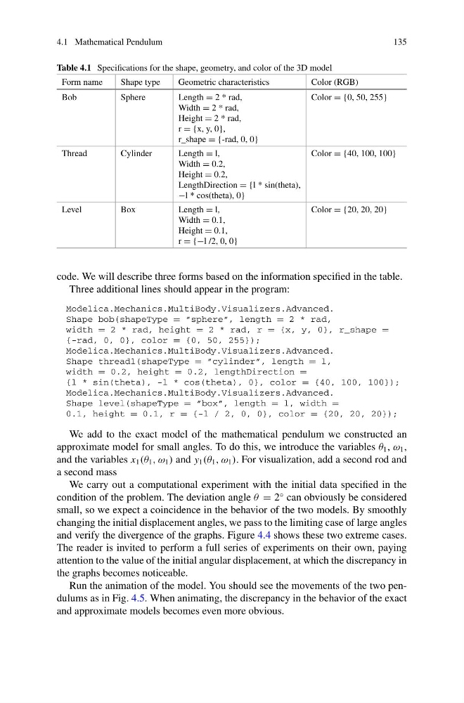
Table 4.1 Specifications for the shape, geometry, and color of the 3D model
Form name
Shape type
Geometric characteristics
Color (RGB)
Bob
Sphere
Length = 2 * rad,
Width = 2 * rad,
Height = 2 * rad,
r = {x, y, 0},
r_shape = {-rad, 0, 0}
Color = {0, 50, 255}
Thread
Cylinder
Length = l,
Width = 0.2,
Height = 0.2,
LengthDirection = {l * sin(theta),
−l * cos(theta), 0}
Color = {40, 100, 100}
Level
Box
Length = l,
Width = 0.1,
Height = 0.1,
r = {−l /2, 0, 0}
Color = {20, 20, 20}
code. We will describe three forms based on the information specified in the table.
Three additional lines should appear in the program:
Modelica.Mechanics.MultiBody.Visualizers.Advanced.
Shape bob(shapeType = ”sphere”, length = 2 * rad,
width = 2 * rad, height = 2 * rad, r = {x, y, 0}, r_shape =
{-rad, 0, 0}, color = {0, 50, 255});
Modelica.Mechanics.MultiBody.Visualizers.Advanced.
Shape thread1(shapeType = ”cylinder”, length = l,
width = 0.2, height = 0.2, lengthDirection =
{l * sin(theta), -l * cos(theta), 0}, color = {40, 100, 100});
Modelica.Mechanics.MultiBody.Visualizers.Advanced.
Shape level(shapeType = ”box”, length = l, width =
0.1, height = 0.1, r = {-l / 2, 0, 0}, color = {20, 20, 20});
We add to the exact model of the mathematical pendulum we constructed an
approximate model for small angles. To do this, we introduce the variables θ 1 , ω 1 ,
and the variables x 1 (θ 1 , ω 1 ) and y 1 (θ 1 , ω 1 ). For visualization, add a second rod and
a second mass
We carry out a computational experiment with the initial data specified in the
condition of the problem. The deviation angle θ = 2
◦ can obviously be considered
small, so we expect a coincidence in the behavior of the two models. By smoothly
changing the initial displacement angles, we pass to the limiting case of large angles
and verify the divergence of the graphs. Figure 4.4 shows these two extreme cases.
The reader is invited to perform a full series of experiments on their own, paying
attention to the value of the initial angular displacement, at which the discrepancy in
the graphs becomes noticeable.
Run the animation of the model. You should see the movements of the two pendulums as in Fig. 4.5. When animating, the discrepancy in the behavior of the exact
and approximate models becomes even more obvious.
135
Table 4.1 Specifications for the shape, geometry, and color of the 3D model
Form name
Shape type
Geometric characteristics
Color (RGB)
Bob
Sphere
Length = 2 * rad,
Width = 2 * rad,
Height = 2 * rad,
r = {x, y, 0},
r_shape = {-rad, 0, 0}
Color = {0, 50, 255}
Thread
Cylinder
Length = l,
Width = 0.2,
Height = 0.2,
LengthDirection = {l * sin(theta),
−l * cos(theta), 0}
Color = {40, 100, 100}
Level
Box
Length = l,
Width = 0.1,
Height = 0.1,
r = {−l /2, 0, 0}
Color = {20, 20, 20}
code. We will describe three forms based on the information specified in the table.
Three additional lines should appear in the program:
Modelica.Mechanics.MultiBody.Visualizers.Advanced.
Shape bob(shapeType = ”sphere”, length = 2 * rad,
width = 2 * rad, height = 2 * rad, r = {x, y, 0}, r_shape =
{-rad, 0, 0}, color = {0, 50, 255});
Modelica.Mechanics.MultiBody.Visualizers.Advanced.
Shape thread1(shapeType = ”cylinder”, length = l,
width = 0.2, height = 0.2, lengthDirection =
{l * sin(theta), -l * cos(theta), 0}, color = {40, 100, 100});
Modelica.Mechanics.MultiBody.Visualizers.Advanced.
Shape level(shapeType = ”box”, length = l, width =
0.1, height = 0.1, r = {-l / 2, 0, 0}, color = {20, 20, 20});
We add to the exact model of the mathematical pendulum we constructed an
approximate model for small angles. To do this, we introduce the variables θ 1 , ω 1 ,
and the variables x 1 (θ 1 , ω 1 ) and y 1 (θ 1 , ω 1 ). For visualization, add a second rod and
a second mass
We carry out a computational experiment with the initial data specified in the
condition of the problem. The deviation angle θ = 2
◦ can obviously be considered
small, so we expect a coincidence in the behavior of the two models. By smoothly
changing the initial displacement angles, we pass to the limiting case of large angles
and verify the divergence of the graphs. Figure 4.4 shows these two extreme cases.
The reader is invited to perform a full series of experiments on their own, paying
attention to the value of the initial angular displacement, at which the discrepancy in
the graphs becomes noticeable.
Run the animation of the model. You should see the movements of the two pendulums as in Fig. 4.5. When animating, the discrepancy in the behavior of the exact
and approximate models becomes even more obvious.