

4.1 Mathematical Pendulum
133
d
2
θ
dt 2 +
g
l
sin θ = 0
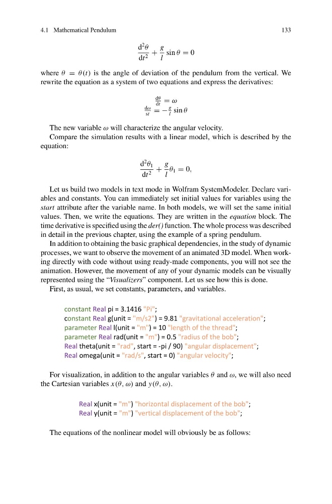
where θ = θ(t) is the angle of deviation of the pendulum from the vertical. We
rewrite the equation as a system of two equations and express the derivatives:
dθ
dt
= ω
dω
st
= −
g
l
sin θ
The new variable ω will characterize the angular velocity.
Compare the simulation results with a linear model, which is described by the
equation:
d
2
θ 1
dt 2 +
g
l
θ 1 = 0,
Let us build two models in text mode in Wolfram SystemModeler. Declare variables and constants. You can immediately set initial values for variables using the
start attribute after the variable name. In both models, we will set the same initial
values. Then, we write the equations. They are written in the equation block. The
time derivative is specified using the der() function. The whole process was described
in detail in the previous chapter, using the example of a spring pendulum.
In addition to obtaining the basic graphical dependencies, in the study of dynamic
processes, we want to observe the movement of an animated 3D model. When working directly with code without using ready-made components, you will not see the
animation. However, the movement of any of your dynamic models can be visually
represented using the “Visualizers” component. Let us see how this is done.
First, as usual, we set constants, parameters, and variables.
constant Real pi = 3.1416 "Pi";
constant Real g(unit = "m/s2") = 9.81 "gravitational acceleration";
parameter Real l(unit = "m") = 10 "length of the thread";
parameter Real rad(unit = "m") = 0.5 "radius of the bob";
Real theta(unit = "rad", start = -pi / 90) "angular displacement";
Real omega(unit = "rad/s", start = 0) "angular velocity";
For visualization, in addition to the angular variables θ and ω, we will also need
the Cartesian variables x(θ, ω) and y(θ, ω).
Real x(unit = "m") "horizontal displacement of the bob";
Real y(unit = "m") "vertical displacement of the bob";
The equations of the nonlinear model will obviously be as follows:
133
d
2
θ
dt 2 +
g
l
sin θ = 0
where θ = θ(t) is the angle of deviation of the pendulum from the vertical. We
rewrite the equation as a system of two equations and express the derivatives:
dθ
dt
= ω
dω
st
= −
g
l
sin θ
The new variable ω will characterize the angular velocity.
Compare the simulation results with a linear model, which is described by the
equation:
d
2
θ 1
dt 2 +
g
l
θ 1 = 0,
Let us build two models in text mode in Wolfram SystemModeler. Declare variables and constants. You can immediately set initial values for variables using the
start attribute after the variable name. In both models, we will set the same initial
values. Then, we write the equations. They are written in the equation block. The
time derivative is specified using the der() function. The whole process was described
in detail in the previous chapter, using the example of a spring pendulum.
In addition to obtaining the basic graphical dependencies, in the study of dynamic
processes, we want to observe the movement of an animated 3D model. When working directly with code without using ready-made components, you will not see the
animation. However, the movement of any of your dynamic models can be visually
represented using the “Visualizers” component. Let us see how this is done.
First, as usual, we set constants, parameters, and variables.
constant Real pi = 3.1416 "Pi";
constant Real g(unit = "m/s2") = 9.81 "gravitational acceleration";
parameter Real l(unit = "m") = 10 "length of the thread";
parameter Real rad(unit = "m") = 0.5 "radius of the bob";
Real theta(unit = "rad", start = -pi / 90) "angular displacement";
Real omega(unit = "rad/s", start = 0) "angular velocity";
For visualization, in addition to the angular variables θ and ω, we will also need
the Cartesian variables x(θ, ω) and y(θ, ω).
Real x(unit = "m") "horizontal displacement of the bob";
Real y(unit = "m") "vertical displacement of the bob";
The equations of the nonlinear model will obviously be as follows: