

3.3 Hierarchical Principles of Model Building
123
d
dt
∂ L
∂ ˙
y
=
d
dt
(m 1 + m 2 ) ˙
y + m 2 l ˙
θ cos θ
= 0
We compose the second Lagrange equation:
∂ L
∂ ˙
θ
= m 2 l
2 ˙
θ + m 2 l ˙
y cos θ
∂ L
∂θ
= −m 2 l
˙
θ ˙
y + g
sin θ
d
dt
∂ L
∂ ˙
θ
= m 2 l
2 ¨
θ + m 2 l ¨
y cos θ − m 2 l ˙
θ ˙
y sin θ
So,
m 2 l
2 ¨
θ + m 2 l ¨
y cos θ + m 2 lg sin θ = 0
As a result, we obtain a system of equations describing the motion of the system
under consideration.
d
dt
(m 1 + m 2 ) ˙
y + m 2 l ˙
θ cos θ
= 0
l ¨
θ + ¨
y cos θ + g sin θ = 0
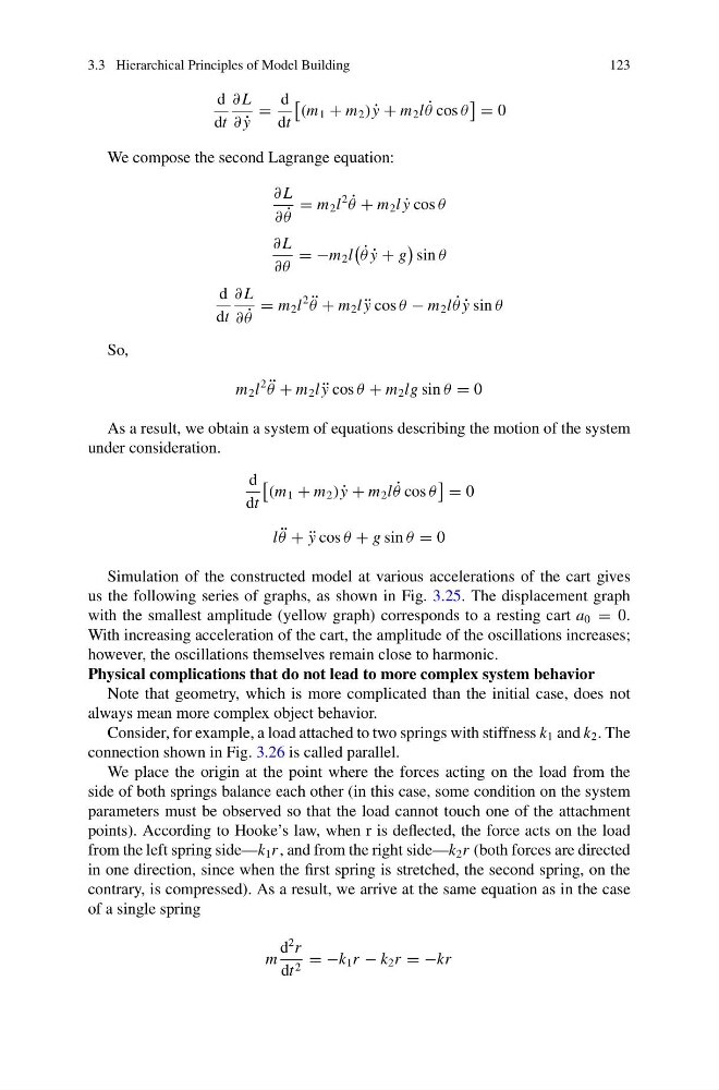
Simulation of the constructed model at various accelerations of the cart gives
us the following series of graphs, as shown in Fig. 3.25. The displacement graph
with the smallest amplitude (yellow graph) corresponds to a resting cart a 0 = 0.
With increasing acceleration of the cart, the amplitude of the oscillations increases;
however, the oscillations themselves remain close to harmonic.
Physical complications that do not lead to more complex system behavior
Note that geometry, which is more complicated than the initial case, does not
always mean more complex object behavior.
Consider, for example, a load attached to two springs with stiffness k 1 and k 2 . The
connection shown in Fig. 3.26 is called parallel.
We place the origin at the point where the forces acting on the load from the
side of both springs balance each other (in this case, some condition on the system
parameters must be observed so that the load cannot touch one of the attachment
points). According to Hooke’s law, when r is deflected, the force acts on the load
from the left spring side—k 1 r , and from the right side—k 2 r (both forces are directed
in one direction, since when the first spring is stretched, the second spring, on the
contrary, is compressed). As a result, we arrive at the same equation as in the case
of a single spring
m
d
2 r
dt 2 = −k 1 r − k 2 r = −kr
123
d
dt
∂ L
∂ ˙
y
=
d
dt
(m 1 + m 2 ) ˙
y + m 2 l ˙
θ cos θ
= 0
We compose the second Lagrange equation:
∂ L
∂ ˙
θ
= m 2 l
2 ˙
θ + m 2 l ˙
y cos θ
∂ L
∂θ
= −m 2 l
˙
θ ˙
y + g
sin θ
d
dt
∂ L
∂ ˙
θ
= m 2 l
2 ¨
θ + m 2 l ¨
y cos θ − m 2 l ˙
θ ˙
y sin θ
So,
m 2 l
2 ¨
θ + m 2 l ¨
y cos θ + m 2 lg sin θ = 0
As a result, we obtain a system of equations describing the motion of the system
under consideration.
d
dt
(m 1 + m 2 ) ˙
y + m 2 l ˙
θ cos θ
= 0
l ¨
θ + ¨
y cos θ + g sin θ = 0
Simulation of the constructed model at various accelerations of the cart gives
us the following series of graphs, as shown in Fig. 3.25. The displacement graph
with the smallest amplitude (yellow graph) corresponds to a resting cart a 0 = 0.
With increasing acceleration of the cart, the amplitude of the oscillations increases;
however, the oscillations themselves remain close to harmonic.
Physical complications that do not lead to more complex system behavior
Note that geometry, which is more complicated than the initial case, does not
always mean more complex object behavior.
Consider, for example, a load attached to two springs with stiffness k 1 and k 2 . The
connection shown in Fig. 3.26 is called parallel.
We place the origin at the point where the forces acting on the load from the
side of both springs balance each other (in this case, some condition on the system
parameters must be observed so that the load cannot touch one of the attachment
points). According to Hooke’s law, when r is deflected, the force acts on the load
from the left spring side—k 1 r , and from the right side—k 2 r (both forces are directed
in one direction, since when the first spring is stretched, the second spring, on the
contrary, is compressed). As a result, we arrive at the same equation as in the case
of a single spring
m
d
2 r
dt 2 = −k 1 r − k 2 r = −kr