

100
3 Computer Simulation of Dynamic Systems
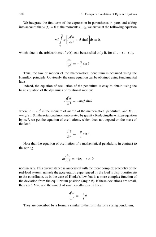
We integrate the first term of the expression in parentheses in parts and taking
into account that ϕ(t) = 0 at the moments t 1 , t 2 , we arrive at the following equation
ml
t 2
t 1
ϕ
l
d
2
θ
dt 2 + d sin θ
dt = 0,
which, due to the arbitrariness of ϕ(t), can be satisfied only if, for all t 1 < t < t 2 ,
d
2
θ
dt 2 = −
g
l
sin θ
Thus, the law of motion of the mathematical pendulum is obtained using the
Hamilton principle. Obviously, the same equation can be obtained using fundamental
laws.
Indeed, the equation of oscillation of the pendulum is easy to obtain using the
basic equation of the dynamics of rotational motion:
J
d
2
θ
dt 2 = −mgl sin θ
where J = ml
2 is the moment of inertia of the mathematical pendulum, and M 1 =
−mgl sin θ is the rotational moment created by gravity. Reducing the written equation
by ml
2 , we get the equation of oscillations, which does not depend on the mass of
the load
d
2
θ
dt 2 = −
g
l
sin θ
Note that the equation of oscillation of a mathematical pendulum, in contrast to
the spring
m
d
2 r
dt 2 = −kr, t > 0
nonlinearly. This circumstance is associated with the more complex geometry of the
rod-load system, namely the acceleration experienced by the load is disproportionate
to the coordinate, as in the case of Hooke’s law, but is a more complex function of
the deviation from the equilibrium position (angle θ ). If these deviations are small,
then sin θ ≈ θ , and the model of small oscillations is linear
d
2
θ
dt 2 = −
g
l
θ
They are described by a formula similar to the formula for a spring pendulum,
3 Computer Simulation of Dynamic Systems
We integrate the first term of the expression in parentheses in parts and taking
into account that ϕ(t) = 0 at the moments t 1 , t 2 , we arrive at the following equation
ml
t 2
t 1
ϕ
l
d
2
θ
dt 2 + d sin θ
dt = 0,
which, due to the arbitrariness of ϕ(t), can be satisfied only if, for all t 1 < t < t 2 ,
d
2
θ
dt 2 = −
g
l
sin θ
Thus, the law of motion of the mathematical pendulum is obtained using the
Hamilton principle. Obviously, the same equation can be obtained using fundamental
laws.
Indeed, the equation of oscillation of the pendulum is easy to obtain using the
basic equation of the dynamics of rotational motion:
J
d
2
θ
dt 2 = −mgl sin θ
where J = ml
2 is the moment of inertia of the mathematical pendulum, and M 1 =
−mgl sin θ is the rotational moment created by gravity. Reducing the written equation
by ml
2 , we get the equation of oscillations, which does not depend on the mass of
the load
d
2
θ
dt 2 = −
g
l
sin θ
Note that the equation of oscillation of a mathematical pendulum, in contrast to
the spring
m
d
2 r
dt 2 = −kr, t > 0
nonlinearly. This circumstance is associated with the more complex geometry of the
rod-load system, namely the acceleration experienced by the load is disproportionate
to the coordinate, as in the case of Hooke’s law, but is a more complex function of
the deviation from the equilibrium position (angle θ ). If these deviations are small,
then sin θ ≈ θ , and the model of small oscillations is linear
d
2
θ
dt 2 = −
g
l
θ
They are described by a formula similar to the formula for a spring pendulum,