

92
3 Computer Simulation of Dynamic Systems
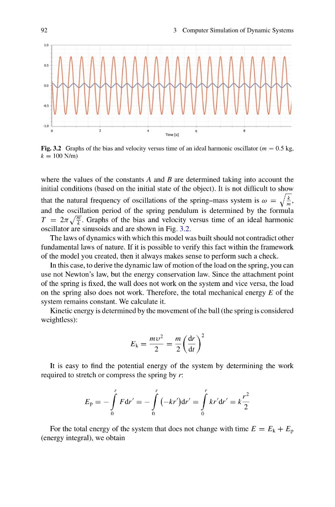
Fig. 3.2 Graphs of the bias and velocity versus time of an ideal harmonic oscillator (m = 0.5 kg,
k = 100 N/m)
where the values of the constants A and B are determined taking into account the
initial conditions (based on the initial state of the object). It is not difficult to show
that the natural frequency of oscillations of the spring–mass system is ω =
k
m
,
and the oscillation period of the spring pendulum is determined by the formula
T = 2π
m
k
. Graphs of the bias and velocity versus time of an ideal harmonic
oscillator are sinusoids and are shown in Fig. 3.2.
The laws of dynamics with which this model was built should not contradict other
fundamental laws of nature. If it is possible to verify this fact within the framework
of the model you created, then it always makes sense to perform such a check.
In this case, to derive the dynamic law of motion of the load on the spring, you can
use not Newton’s law, but the energy conservation law. Since the attachment point
of the spring is fixed, the wall does not work on the system and vice versa, the load
on the spring also does not work. Therefore, the total mechanical energy E of the
system remains constant. We calculate it.
Kinetic energy is determined by the movement of the ball (the spring is considered
weightless):
E k =
mυ
2
2
=
m
2
dr
dt
2
It is easy to find the potential energy of the system by determining the work
required to stretch or compress the spring by r:
E p = −
r
0
Fdr
= −
r
0
−kr
dr
=
r
0
kr
dr
= k
r
2
2
For the total energy of the system that does not change with time E = E k + E p
(energy integral), we obtain
3 Computer Simulation of Dynamic Systems
Fig. 3.2 Graphs of the bias and velocity versus time of an ideal harmonic oscillator (m = 0.5 kg,
k = 100 N/m)
where the values of the constants A and B are determined taking into account the
initial conditions (based on the initial state of the object). It is not difficult to show
that the natural frequency of oscillations of the spring–mass system is ω =
k
m
,
and the oscillation period of the spring pendulum is determined by the formula
T = 2π
m
k
. Graphs of the bias and velocity versus time of an ideal harmonic
oscillator are sinusoids and are shown in Fig. 3.2.
The laws of dynamics with which this model was built should not contradict other
fundamental laws of nature. If it is possible to verify this fact within the framework
of the model you created, then it always makes sense to perform such a check.
In this case, to derive the dynamic law of motion of the load on the spring, you can
use not Newton’s law, but the energy conservation law. Since the attachment point
of the spring is fixed, the wall does not work on the system and vice versa, the load
on the spring also does not work. Therefore, the total mechanical energy E of the
system remains constant. We calculate it.
Kinetic energy is determined by the movement of the ball (the spring is considered
weightless):
E k =
mυ
2
2
=
m
2
dr
dt
2
It is easy to find the potential energy of the system by determining the work
required to stretch or compress the spring by r:
E p = −
r
0
Fdr
= −
r
0
−kr
dr
=
r
0
kr
dr
= k
r
2
2
For the total energy of the system that does not change with time E = E k + E p
(energy integral), we obtain