

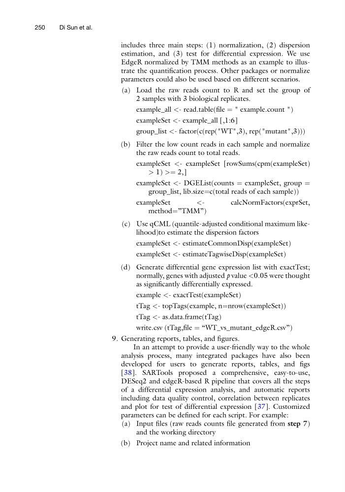
includes three main steps: (1) normalization, (2) dispersion
estimation, and (3) test for differential expression. We use
EdgeR normalized by TMM methods as an example to illustrate the quantification process. Other packages or normalize
parameters could also be used based on different scenarios.
(a) Load the raw reads count to R and set the group of
2 samples with 3 biological replicates.
example_all <- read.table(file ¼ " example.count ")
exampleSet <- example_all [,1:6]
group_list <- factor(c(rep("WT",3), rep("mutant",3)))
(b) Filter the low count reads in each sample and normalize
the raw reads count to total reads.
exampleSet <- exampleSet [rowSums(cpm(exampleSet)
> 1) >¼ 2,]
exampleSet <- DGEList(counts ¼ exampleSet, group ¼
group_list, lib.size¼c(total reads of each sample))
exampleSet
(c) Use qCML (quantile-adjusted conditional maximum likelihood)to estimate the dispersion factors
exampleSet <- estimateCommonDisp(exampleSet)
exampleSet <- estimateTagwiseDisp(exampleSet)
(d) Generate differential gene expression list with exactTest;
normally, genes with adjusted p value <0.05 were thought
as significantly differentially expressed.
example <- exactTest(exampleSet)
tTag <- topTags(example, n¼nrow(exampleSet))
tTag <- as.data.frame(tTag)
write.csv (tTag,file ¼ “WT_vs_mutant_edgeR.csv”)
9. Generating reports, tables, and figures.
In an attempt to provide a user-friendly way to the whole
analysis process, many integrated packages have also been
developed for users to generate reports, tables, and figs
[38]. SARTools proposed a comprehensive, easy-to-use,
DESeq2 and edgeR-based R pipeline that covers all the steps
of a differential expression analysis, and automatic reports
including data quality control, correlation between replicates
and plot for test of differential expression [37]. Customized
parameters can be defined for each script. For example:
(a) Input files (raw reads counts file generated from step 7)
and the working directory
(b) Project name and related information
250
Di Sun et al.
estimation, and (3) test for differential expression. We use
EdgeR normalized by TMM methods as an example to illustrate the quantification process. Other packages or normalize
parameters could also be used based on different scenarios.
(a) Load the raw reads count to R and set the group of
2 samples with 3 biological replicates.
example_all <- read.table(file ¼ " example.count ")
exampleSet <- example_all [,1:6]
group_list <- factor(c(rep("WT",3), rep("mutant",3)))
(b) Filter the low count reads in each sample and normalize
the raw reads count to total reads.
exampleSet <- exampleSet [rowSums(cpm(exampleSet)
> 1) >¼ 2,]
exampleSet <- DGEList(counts ¼ exampleSet, group ¼
group_list, lib.size¼c(total reads of each sample))
exampleSet
(c) Use qCML (quantile-adjusted conditional maximum likelihood)to estimate the dispersion factors
exampleSet <- estimateCommonDisp(exampleSet)
exampleSet <- estimateTagwiseDisp(exampleSet)
(d) Generate differential gene expression list with exactTest;
normally, genes with adjusted p value <0.05 were thought
as significantly differentially expressed.
example <- exactTest(exampleSet)
tTag <- topTags(example, n¼nrow(exampleSet))
tTag <- as.data.frame(tTag)
write.csv (tTag,file ¼ “WT_vs_mutant_edgeR.csv”)
9. Generating reports, tables, and figures.
In an attempt to provide a user-friendly way to the whole
analysis process, many integrated packages have also been
developed for users to generate reports, tables, and figs
[38]. SARTools proposed a comprehensive, easy-to-use,
DESeq2 and edgeR-based R pipeline that covers all the steps
of a differential expression analysis, and automatic reports
including data quality control, correlation between replicates
and plot for test of differential expression [37]. Customized
parameters can be defined for each script. For example:
(a) Input files (raw reads counts file generated from step 7)
and the working directory
(b) Project name and related information
250
Di Sun et al.