

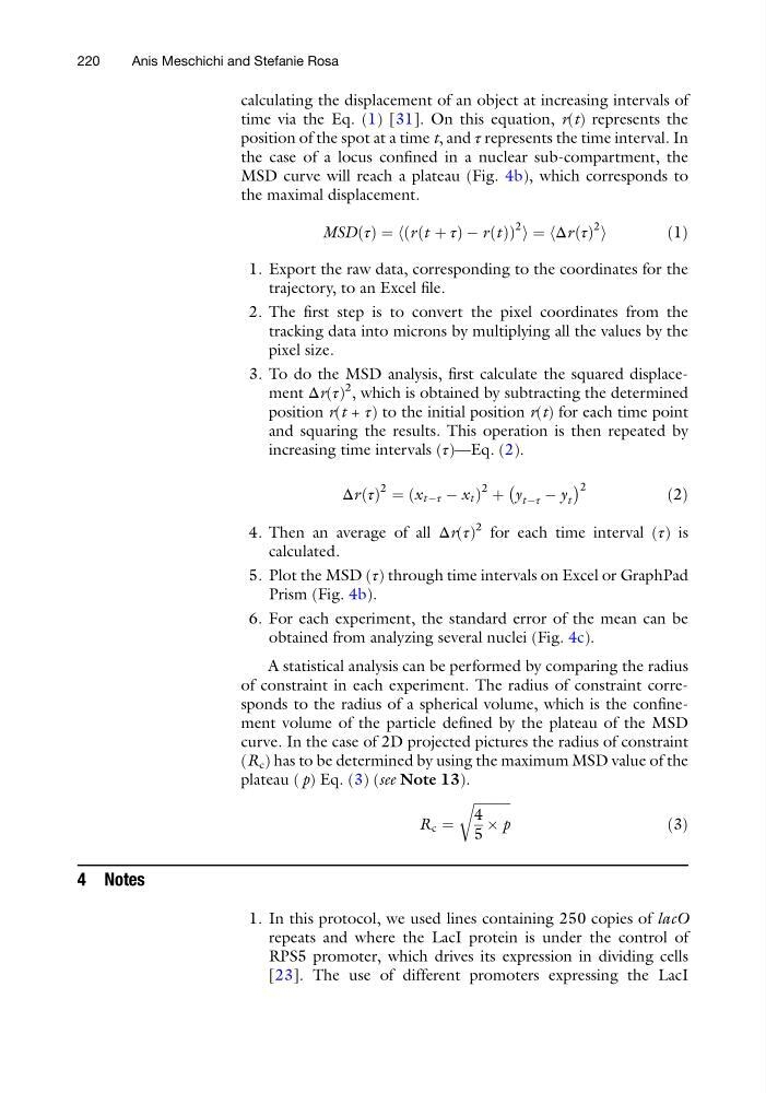
calculating the displacement of an object at increasing intervals of
time via the Eq. (1) [31]. On this equation, r(t) represents the
position of the spot at a time t, and τ represents the time interval. In
the case of a locus confined in a nuclear sub-compartment, the
MSD curve will reach a plateau (Fig. 4b), which corresponds to
the maximal displacement.
MSD τ
ð Þ ¼ h r t þ τ
ð
ÞÀr t
ð Þ
ð
Þ
2 i ¼ hΔr τ
ð Þ
2 i
ð 1Þ
1. Export the raw data, corresponding to the coordinates for the
trajectory, to an Excel file.
2. The first step is to convert the pixel coordinates from the
tracking data into microns by multiplying all the values by the
pixel size.
3. To do the MSD analysis, first calculate the squared displacement Δr(τ)
2 , which is obtained by subtracting the determined
position r(t + τ) to the initial position r(t) for each time point
and squaring the results. This operation is then repeated by
increasing time intervals (τ)—Eq. (2).
Δr τ
ð Þ
2 ¼ x tÀτ À x t
ð
Þ
2 þ y tÀτ À y t
À
Á 2
ð2Þ
4. Then an average of all Δr(τ)
2 for each time interval (τ) is
calculated.
5. Plot the MSD (τ) through time intervals on Excel or GraphPad
Prism (Fig. 4b).
6. For each experiment, the standard error of the mean can be
obtained from analyzing several nuclei (Fig. 4c).
A statistical analysis can be performed by comparing the radius
of constraint in each experiment. The radius of constraint corresponds to the radius of a spherical volume, which is the confinement volume of the particle defined by the plateau of the MSD
curve. In the case of 2D projected pictures the radius of constraint
(R c ) has to be determined by using the maximum MSD value of the
plateau ( p) Eq. (3) (see Note 13).
R c ¼
ffiffiffiffiffiffiffiffiffiffiffi
4
5
 p
r
ð3Þ
4 Notes
1. In this protocol, we used lines containing 250 copies of lacO
repeats and where the LacI protein is under the control of
RPS5 promoter, which drives its expression in dividing cells
[23]. The use of different promoters expressing the LacI
220
Anis Meschichi and Stefanie Rosa
time via the Eq. (1) [31]. On this equation, r(t) represents the
position of the spot at a time t, and τ represents the time interval. In
the case of a locus confined in a nuclear sub-compartment, the
MSD curve will reach a plateau (Fig. 4b), which corresponds to
the maximal displacement.
MSD τ
ð Þ ¼ h r t þ τ
ð
ÞÀr t
ð Þ
ð
Þ
2 i ¼ hΔr τ
ð Þ
2 i
ð 1Þ
1. Export the raw data, corresponding to the coordinates for the
trajectory, to an Excel file.
2. The first step is to convert the pixel coordinates from the
tracking data into microns by multiplying all the values by the
pixel size.
3. To do the MSD analysis, first calculate the squared displacement Δr(τ)
2 , which is obtained by subtracting the determined
position r(t + τ) to the initial position r(t) for each time point
and squaring the results. This operation is then repeated by
increasing time intervals (τ)—Eq. (2).
Δr τ
ð Þ
2 ¼ x tÀτ À x t
ð
Þ
2 þ y tÀτ À y t
À
Á 2
ð2Þ
4. Then an average of all Δr(τ)
2 for each time interval (τ) is
calculated.
5. Plot the MSD (τ) through time intervals on Excel or GraphPad
Prism (Fig. 4b).
6. For each experiment, the standard error of the mean can be
obtained from analyzing several nuclei (Fig. 4c).
A statistical analysis can be performed by comparing the radius
of constraint in each experiment. The radius of constraint corresponds to the radius of a spherical volume, which is the confinement volume of the particle defined by the plateau of the MSD
curve. In the case of 2D projected pictures the radius of constraint
(R c ) has to be determined by using the maximum MSD value of the
plateau ( p) Eq. (3) (see Note 13).
R c ¼
ffiffiffiffiffiffiffiffiffiffiffi
4
5
 p
r
ð3Þ
4 Notes
1. In this protocol, we used lines containing 250 copies of lacO
repeats and where the LacI protein is under the control of
RPS5 promoter, which drives its expression in dividing cells
[23]. The use of different promoters expressing the LacI
220
Anis Meschichi and Stefanie Rosa