

3. Format the input data.
>library(stringr) #no need to install stringr
>sep_ps<-str_split_fixed(ps$SNP,'_',2)
>chr<-as.numeric(sep_ps[,1])
>base<-as.numeric(sep_ps[,2])
>dat<-as.data.frame(cbind(chr,base,ps$pvalue))
>colnames(dat)<-c('CHR','BP','P')
4. Plot the input data.
>png(file='glucose_emmax_manhattanplot.png',width=20,height=12,units='in',res=500)
>par(mar=c(6.1,6.1,2.1,2.1))
>manhattan(dat,suggestiveline=F,genomewideline=F)
>dev.off()
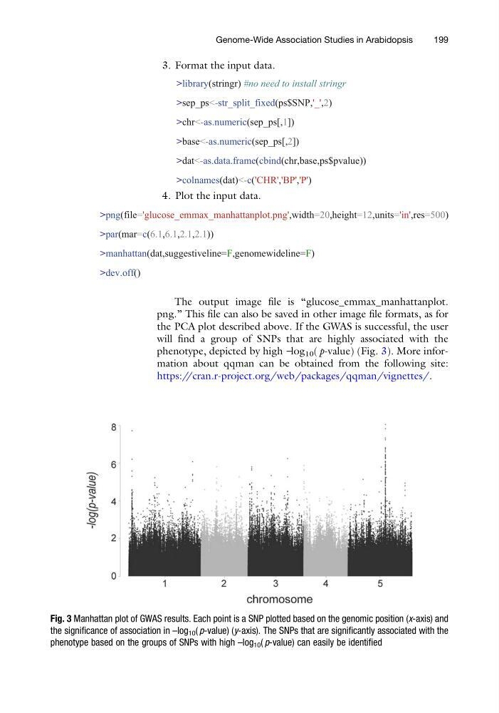
The output image file is “glucose_emmax_manhattanplot.
png.” This file can also be saved in other image file formats, as for
the PCA plot described above. If the GWAS is successful, the user
will find a group of SNPs that are highly associated with the
phenotype, depicted by high –log 10 ( p-value) (Fig. 3). More information about qqman can be obtained from the following site:
https://cran.r-project.org/web/packages/qqman/vignettes/.
Fig. 3 Manhattan plot of GWAS results. Each point is a SNP plotted based on the genomic position (x-axis) and
the significance of association in –log 10 ( p-value) (y-axis). The SNPs that are significantly associated with the
phenotype based on the groups of SNPs with high –log 10 ( p-value) can easily be identified
Genome-Wide Association Studies in Arabidopsis
199
>library(stringr) #no need to install stringr
>sep_ps<-str_split_fixed(ps$SNP,'_',2)
>chr<-as.numeric(sep_ps[,1])
>base<-as.numeric(sep_ps[,2])
>dat<-as.data.frame(cbind(chr,base,ps$pvalue))
>colnames(dat)<-c('CHR','BP','P')
4. Plot the input data.
>png(file='glucose_emmax_manhattanplot.png',width=20,height=12,units='in',res=500)
>par(mar=c(6.1,6.1,2.1,2.1))
>manhattan(dat,suggestiveline=F,genomewideline=F)
>dev.off()
The output image file is “glucose_emmax_manhattanplot.
png.” This file can also be saved in other image file formats, as for
the PCA plot described above. If the GWAS is successful, the user
will find a group of SNPs that are highly associated with the
phenotype, depicted by high –log 10 ( p-value) (Fig. 3). More information about qqman can be obtained from the following site:
https://cran.r-project.org/web/packages/qqman/vignettes/.
Fig. 3 Manhattan plot of GWAS results. Each point is a SNP plotted based on the genomic position (x-axis) and
the significance of association in –log 10 ( p-value) (y-axis). The SNPs that are significantly associated with the
phenotype based on the groups of SNPs with high –log 10 ( p-value) can easily be identified
Genome-Wide Association Studies in Arabidopsis
199