

U ¼
1
2
X K
j;k¼1
Q j Q k
X K
l;m¼1
a lj F lm a mk :
ð2:52Þ
Since
P K
l;m¼1 a lj F lm a mk ¼ m
2
j d jk (see, e.g., [5]), we obtain
U ¼
1
2
X K
j¼1
Q
2
j
X K
l;m¼1
a lj F lm a mj :
ð2:53Þ
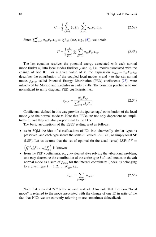
The last equation resolves the potential energy associated with each normal
mode (index j) into local modes (indices l and m), i.e., modes associated with the
change of one IC. For a given value of j, the expression p lm;j ¼ a lj F lm a mj
describes the contribution of the coupled local modes l and m to the jth normal
mode. p lm;j , called Potential Energy Distribution (PED) coefficients [73], were
introduced by Morino and Kuchitsu in early 1950s. The common practice is to use
normalized to unity diagonal PED coefficients, i.e.,
p ll;j ¼
a
2
lj F ll
P K
m¼1 a 2
mj F mm
:
ð2:54Þ
Coefficients defined in this way provide the (percentage) contribution of the local
mode l to the normal mode j. Note that PEDs are not only dependent on amplitudes a, and they are also proportional to the FCs.
The basic assumptions of the ESFF scaling read as follows:
• as in SQM the idea of classifications of ICs into chemically similar types is
preserved, and each type shares the same SF called ESFF SF, or simply local SF
(LSF). Let us assume that the set of optimal (in the usual sense) LSFs f
opt
¼
f
opt
1 ; f
opt
2 ; . . .; f
opt
N typ
is known;
• from the PED coefficients, p ll;j , evaluated after solving the vibrational problem,
one may determine the contribution of the entire type I of local modes to the jth
normal mode as a sum of p ll;j for the internal coordinates (index l) belonging
to a given type I ¼ 1; 2; . . .; N typ , i.e.,
P I;j ¼
X
l2typeI
p ll;j :
ð2:55Þ
Note that a capital “P” letter is used instead. Also note that the term “local
mode” is referred to the mode associated with the change of one IC in spite of the
fact that NICs we are currently referring to are sometimes delocalized;
82
O. Bąk and P. Borowski
1
2
X K
j;k¼1
Q j Q k
X K
l;m¼1
a lj F lm a mk :
ð2:52Þ
Since
P K
l;m¼1 a lj F lm a mk ¼ m
2
j d jk (see, e.g., [5]), we obtain
U ¼
1
2
X K
j¼1
Q
2
j
X K
l;m¼1
a lj F lm a mj :
ð2:53Þ
The last equation resolves the potential energy associated with each normal
mode (index j) into local modes (indices l and m), i.e., modes associated with the
change of one IC. For a given value of j, the expression p lm;j ¼ a lj F lm a mj
describes the contribution of the coupled local modes l and m to the jth normal
mode. p lm;j , called Potential Energy Distribution (PED) coefficients [73], were
introduced by Morino and Kuchitsu in early 1950s. The common practice is to use
normalized to unity diagonal PED coefficients, i.e.,
p ll;j ¼
a
2
lj F ll
P K
m¼1 a 2
mj F mm
:
ð2:54Þ
Coefficients defined in this way provide the (percentage) contribution of the local
mode l to the normal mode j. Note that PEDs are not only dependent on amplitudes a, and they are also proportional to the FCs.
The basic assumptions of the ESFF scaling read as follows:
• as in SQM the idea of classifications of ICs into chemically similar types is
preserved, and each type shares the same SF called ESFF SF, or simply local SF
(LSF). Let us assume that the set of optimal (in the usual sense) LSFs f
opt
¼
f
opt
1 ; f
opt
2 ; . . .; f
opt
N typ
is known;
• from the PED coefficients, p ll;j , evaluated after solving the vibrational problem,
one may determine the contribution of the entire type I of local modes to the jth
normal mode as a sum of p ll;j for the internal coordinates (index l) belonging
to a given type I ¼ 1; 2; . . .; N typ , i.e.,
P I;j ¼
X
l2typeI
p ll;j :
ð2:55Þ
Note that a capital “P” letter is used instead. Also note that the term “local
mode” is referred to the mode associated with the change of one IC in spite of the
fact that NICs we are currently referring to are sometimes delocalized;
82
O. Bąk and P. Borowski