

considerably lower computational requirements, resulting in increasing number of
studies published in recent years devoted to TD-DFT application for the analysis of
various systems in excited states and related absorption and emission processes.
Despite some objections to the TD-DFT method, e.g., lack of equal precision for
electronic transitions of various nature, incorrect description of long-range dispersive forces by standard functionals, an over-polarization problem, limited precision
of the description of induced delocalized states (molecular valence states with
extended p systems, Rydberg states, and doubly excited states), a problem with the
selection of a suitable functional and basis function set (the results obtained with
their use should be verified based on available experimental data) [102, 107, 108,
110], due to very large computational requirements in the case of correlated wave
function-based post-HF methods, TD-DFT based methods (thanks to the ability to
deliver good quantitative results for medium-sized systems at reasonably low
computational costs) have become very popular in simulations of excited
properties. Given the above, it seems that currently TD-DFT is arguably the best
compromise between precision and computational costs for modeling and analyzing
the properties of excited states of medium and larger molecular and periodic systems. Therefore, in the following paragraphs, the basic assumptions of this method
will be presented.
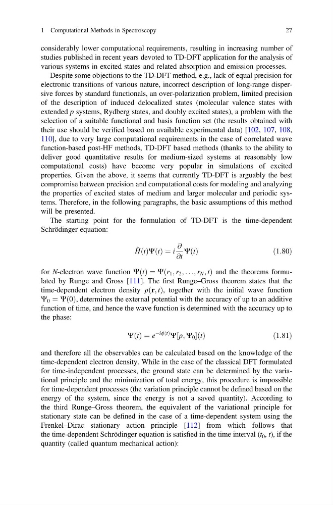
The starting point for the formulation of TD-DFT is the time-dependent
Schrödinger equation:
^
H t
ð ÞW t
ð Þ ¼ i
@
@t
W t
ð Þ
ð1:80Þ
for N-electron wave function W t
ð Þ ¼ W r 1 ; r 2 ; . . .; r N ; t
ð
Þand the theorems formulated by Runge and Gross [111]. The first Runge–Gross theorem states that the
time-dependent electron density q r; t
ð Þ, together with the initial wave function
W 0 ¼ W 0
ð Þ, determines the external potential with the accuracy of up to an additive
function of time, and hence the wave function is determined with the accuracy up to
the phase:
WðtÞ ¼ e
Ài/ðtÞ
W½q; W 0 ðtÞ
ð 1:81Þ
and therefore all the observables can be calculated based on the knowledge of the
time-dependent electron density. While in the case of the classical DFT formulated
for time-independent processes, the ground state can be determined by the variational principle and the minimization of total energy, this procedure is impossible
for time-dependent processes (the variation principle cannot be defined based on the
energy of the system, since the energy is not a saved quantity). According to
the third Runge–Gross theorem, the equivalent of the variational principle for
stationary state can be defined in the case of a time-dependent system using the
Frenkel–Dirac stationary action principle [112] from which follows that
the time-dependent Schrödinger equation is satisfied in the time interval (t 0 , t), if the
quantity (called quantum mechanical action):
1 Computational Methods in Spectroscopy
27
studies published in recent years devoted to TD-DFT application for the analysis of
various systems in excited states and related absorption and emission processes.
Despite some objections to the TD-DFT method, e.g., lack of equal precision for
electronic transitions of various nature, incorrect description of long-range dispersive forces by standard functionals, an over-polarization problem, limited precision
of the description of induced delocalized states (molecular valence states with
extended p systems, Rydberg states, and doubly excited states), a problem with the
selection of a suitable functional and basis function set (the results obtained with
their use should be verified based on available experimental data) [102, 107, 108,
110], due to very large computational requirements in the case of correlated wave
function-based post-HF methods, TD-DFT based methods (thanks to the ability to
deliver good quantitative results for medium-sized systems at reasonably low
computational costs) have become very popular in simulations of excited
properties. Given the above, it seems that currently TD-DFT is arguably the best
compromise between precision and computational costs for modeling and analyzing
the properties of excited states of medium and larger molecular and periodic systems. Therefore, in the following paragraphs, the basic assumptions of this method
will be presented.
The starting point for the formulation of TD-DFT is the time-dependent
Schrödinger equation:
^
H t
ð ÞW t
ð Þ ¼ i
@
@t
W t
ð Þ
ð1:80Þ
for N-electron wave function W t
ð Þ ¼ W r 1 ; r 2 ; . . .; r N ; t
ð
Þand the theorems formulated by Runge and Gross [111]. The first Runge–Gross theorem states that the
time-dependent electron density q r; t
ð Þ, together with the initial wave function
W 0 ¼ W 0
ð Þ, determines the external potential with the accuracy of up to an additive
function of time, and hence the wave function is determined with the accuracy up to
the phase:
WðtÞ ¼ e
Ài/ðtÞ
W½q; W 0 ðtÞ
ð 1:81Þ
and therefore all the observables can be calculated based on the knowledge of the
time-dependent electron density. While in the case of the classical DFT formulated
for time-independent processes, the ground state can be determined by the variational principle and the minimization of total energy, this procedure is impossible
for time-dependent processes (the variation principle cannot be defined based on the
energy of the system, since the energy is not a saved quantity). According to
the third Runge–Gross theorem, the equivalent of the variational principle for
stationary state can be defined in the case of a time-dependent system using the
Frenkel–Dirac stationary action principle [112] from which follows that
the time-dependent Schrödinger equation is satisfied in the time interval (t 0 , t), if the
quantity (called quantum mechanical action):
1 Computational Methods in Spectroscopy
27