

the parameters for last over 20 years. The parameters have been calculated using
coupled-cluster (CC) theory, density functional theory (DFT), full linearized plane
waves (FLAPW) method, Hartree–Fock (HF) and with the application of different
basis functions, exchange-correlation potentials, etc. [13]. While most of the
methods work well for the vast majority of solids, they may fail for so-called
correlated electrons in 3d transition metal oxides or 4f and 5f compounds.
Unfortunately, iron belongs often to this class of materials and prediction of its
electronic structure may not be so reliable. Except for the problem of treating the
electron–electron interaction, there is a problem which magnetic order should be
considered (paramagnetic, ferromagnetic, different antiferromagnetic or ferrimagnetic configurations) or whether the relativistic effects should be included, e.g.,
orbital contribution in the magnetic hyperfine field [14–16].
One of the most frequently calculated hyperfine interaction parameter is the
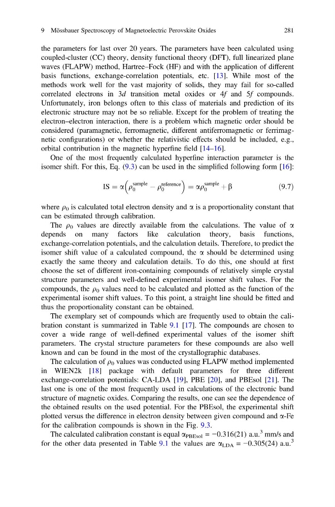
isomer shift. For this, Eq. (9.3) can be used in the simplified following form [16]:
IS ¼ a q
sample
0
À q
reference
0
¼ aq
sample
0
þ b
ð9:7Þ
where q 0 is calculated total electron density and a is a proportionality constant that
can be estimated through calibration.
The q 0 values are directly available from the calculations. The value of a
depends on many factors like calculation theory, basis functions,
exchange-correlation potentials, and the calculation details. Therefore, to predict the
isomer shift value of a calculated compound, the a should be determined using
exactly the same theory and calculation details. To do this, one should at first
choose the set of different iron-containing compounds of relatively simple crystal
structure parameters and well-defined experimental isomer shift values. For the
compounds, the q 0 values need to be calculated and plotted as the function of the
experimental isomer shift values. To this point, a straight line should be fitted and
thus the proportionality constant can be obtained.
The exemplary set of compounds which are frequently used to obtain the calibration constant is summarized in Table 9.1 [17]. The compounds are chosen to
cover a wide range of well-defined experimental values of the isomer shift
parameters. The crystal structure parameters for these compounds are also well
known and can be found in the most of the crystallographic databases.
The calculation of q 0 values was conducted using FLAPW method implemented
in WIEN2k [18] package with default parameters for three different
exchange-correlation potentials: CA-LDA [19], PBE [20], and PBEsol [21]. The
last one is one of the most frequently used in calculations of the electronic band
structure of magnetic oxides. Comparing the results, one can see the dependence of
the obtained results on the used potential. For the PBEsol, the experimental shift
plotted versus the difference in electron density between given compound and a-Fe
for the calibration compounds is shown in the Fig. 9.3.
The calculated calibration constant is equal a PBEsol = −0.316(21) a.u.
3 mm/s and
for the other data presented in Table 9.1 the values are a LDA = −0.305(24) a.u.
3
9 Mössbauer Spectroscopy of Magnetoelectric Perovskite Oxides
281
coupled-cluster (CC) theory, density functional theory (DFT), full linearized plane
waves (FLAPW) method, Hartree–Fock (HF) and with the application of different
basis functions, exchange-correlation potentials, etc. [13]. While most of the
methods work well for the vast majority of solids, they may fail for so-called
correlated electrons in 3d transition metal oxides or 4f and 5f compounds.
Unfortunately, iron belongs often to this class of materials and prediction of its
electronic structure may not be so reliable. Except for the problem of treating the
electron–electron interaction, there is a problem which magnetic order should be
considered (paramagnetic, ferromagnetic, different antiferromagnetic or ferrimagnetic configurations) or whether the relativistic effects should be included, e.g.,
orbital contribution in the magnetic hyperfine field [14–16].
One of the most frequently calculated hyperfine interaction parameter is the
isomer shift. For this, Eq. (9.3) can be used in the simplified following form [16]:
IS ¼ a q
sample
0
À q
reference
0
¼ aq
sample
0
þ b
ð9:7Þ
where q 0 is calculated total electron density and a is a proportionality constant that
can be estimated through calibration.
The q 0 values are directly available from the calculations. The value of a
depends on many factors like calculation theory, basis functions,
exchange-correlation potentials, and the calculation details. Therefore, to predict the
isomer shift value of a calculated compound, the a should be determined using
exactly the same theory and calculation details. To do this, one should at first
choose the set of different iron-containing compounds of relatively simple crystal
structure parameters and well-defined experimental isomer shift values. For the
compounds, the q 0 values need to be calculated and plotted as the function of the
experimental isomer shift values. To this point, a straight line should be fitted and
thus the proportionality constant can be obtained.
The exemplary set of compounds which are frequently used to obtain the calibration constant is summarized in Table 9.1 [17]. The compounds are chosen to
cover a wide range of well-defined experimental values of the isomer shift
parameters. The crystal structure parameters for these compounds are also well
known and can be found in the most of the crystallographic databases.
The calculation of q 0 values was conducted using FLAPW method implemented
in WIEN2k [18] package with default parameters for three different
exchange-correlation potentials: CA-LDA [19], PBE [20], and PBEsol [21]. The
last one is one of the most frequently used in calculations of the electronic band
structure of magnetic oxides. Comparing the results, one can see the dependence of
the obtained results on the used potential. For the PBEsol, the experimental shift
plotted versus the difference in electron density between given compound and a-Fe
for the calibration compounds is shown in the Fig. 9.3.
The calculated calibration constant is equal a PBEsol = −0.316(21) a.u.
3 mm/s and
for the other data presented in Table 9.1 the values are a LDA = −0.305(24) a.u.
3
9 Mössbauer Spectroscopy of Magnetoelectric Perovskite Oxides
281