

50
4 Sefficiency (Sustainable Efficiency)
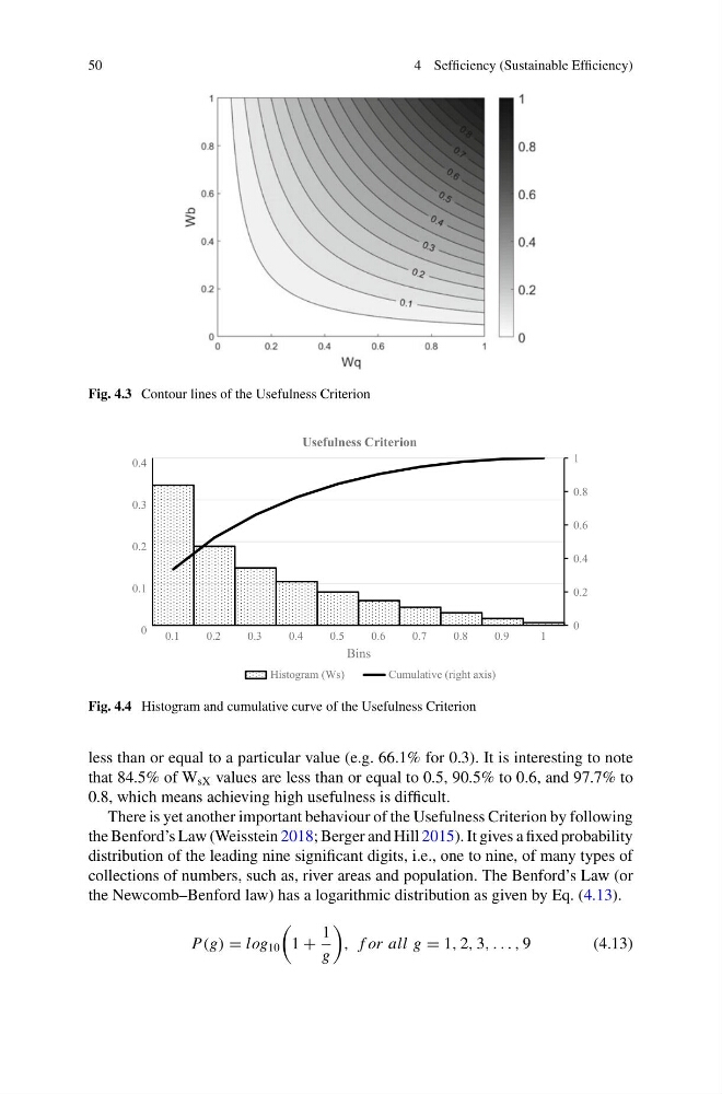
Fig. 4.3 Contour lines of the Usefulness Criterion
0
0.2
0.4
0.6
0.8
1
0
0.1
0.2
0.3
0.4
0.1
0.2
0.3
0.4
0.5
0.6
0.7
0.8
0.9
1
Bins
Usefulness Criterion
Histogram (Ws)
Cumulative (right axis)
Fig. 4.4 Histogram and cumulative curve of the Usefulness Criterion
less than or equal to a particular value (e.g. 66.1% for 0.3). It is interesting to note
that 84.5% of W sX values are less than or equal to 0.5, 90.5% to 0.6, and 97.7% to
0.8, which means achieving high usefulness is difficult.
There is yet another important behaviour of the Usefulness Criterion by following
the Benford’s Law (Weisstein 2018; Berger and Hill 2015). It gives a fixed probability
distribution of the leading nine significant digits, i.e., one to nine, of many types of
collections of numbers, such as, river areas and population. The Benford’s Law (or
the Newcomb–Benford law) has a logarithmic distribution as given by Eq. (4.13).
P(g) = log 10
1 +
1
g
, f or all g = 1, 2, 3, . . . , 9
(4.13)
4 Sefficiency (Sustainable Efficiency)
Fig. 4.3 Contour lines of the Usefulness Criterion
0
0.2
0.4
0.6
0.8
1
0
0.1
0.2
0.3
0.4
0.1
0.2
0.3
0.4
0.5
0.6
0.7
0.8
0.9
1
Bins
Usefulness Criterion
Histogram (Ws)
Cumulative (right axis)
Fig. 4.4 Histogram and cumulative curve of the Usefulness Criterion
less than or equal to a particular value (e.g. 66.1% for 0.3). It is interesting to note
that 84.5% of W sX values are less than or equal to 0.5, 90.5% to 0.6, and 97.7% to
0.8, which means achieving high usefulness is difficult.
There is yet another important behaviour of the Usefulness Criterion by following
the Benford’s Law (Weisstein 2018; Berger and Hill 2015). It gives a fixed probability
distribution of the leading nine significant digits, i.e., one to nine, of many types of
collections of numbers, such as, river areas and population. The Benford’s Law (or
the Newcomb–Benford law) has a logarithmic distribution as given by Eq. (4.13).
P(g) = log 10
1 +
1
g
, f or all g = 1, 2, 3, . . . , 9
(4.13)