

4.3 Weights
49
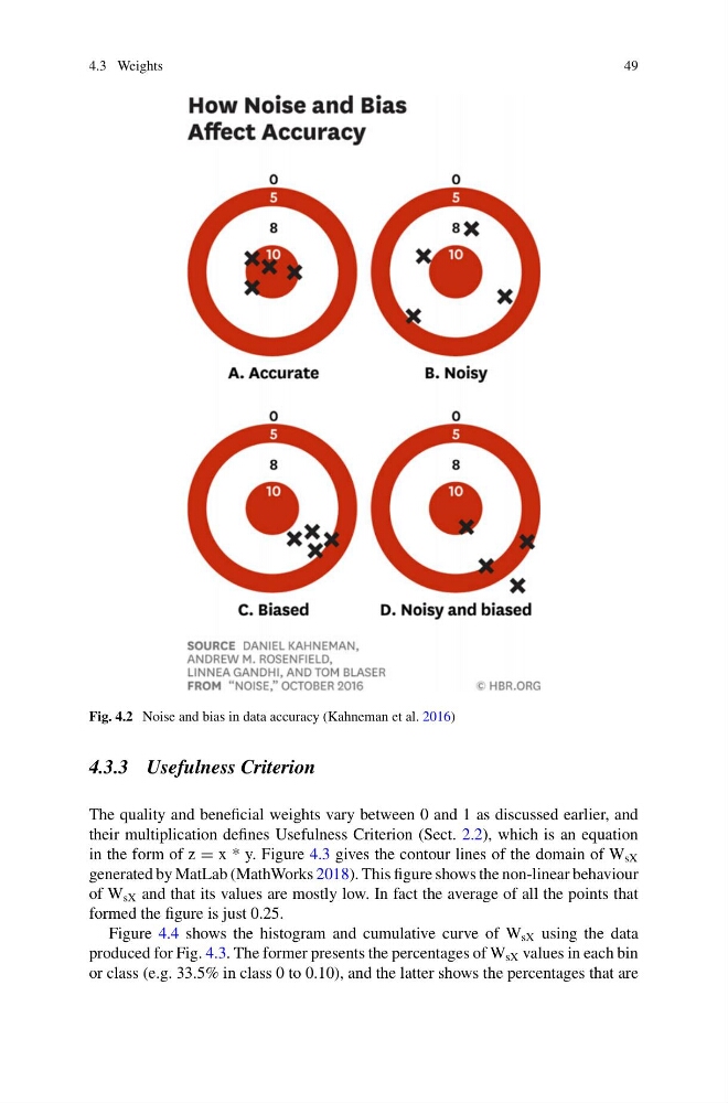
Fig. 4.2 Noise and bias in data accuracy (Kahneman et al. 2016)
4.3.3 Usefulness Criterion
The quality and beneficial weights vary between 0 and 1 as discussed earlier, and
their multiplication defines Usefulness Criterion (Sect. 2.2), which is an equation
in the form of z = x * y. Figure 4.3 gives the contour lines of the domain of W sX
generated by MatLab (MathWorks 2018). This figure shows the non-linear behaviour
of W sX and that its values are mostly low. In fact the average of all the points that
formed the figure is just 0.25.
Figure 4.4 shows the histogram and cumulative curve of W sX using the data
produced for Fig. 4.3. The former presents the percentages of W sX values in each bin
or class (e.g. 33.5% in class 0 to 0.10), and the latter shows the percentages that are
49
Fig. 4.2 Noise and bias in data accuracy (Kahneman et al. 2016)
4.3.3 Usefulness Criterion
The quality and beneficial weights vary between 0 and 1 as discussed earlier, and
their multiplication defines Usefulness Criterion (Sect. 2.2), which is an equation
in the form of z = x * y. Figure 4.3 gives the contour lines of the domain of W sX
generated by MatLab (MathWorks 2018). This figure shows the non-linear behaviour
of W sX and that its values are mostly low. In fact the average of all the points that
formed the figure is just 0.25.
Figure 4.4 shows the histogram and cumulative curve of W sX using the data
produced for Fig. 4.3. The former presents the percentages of W sX values in each bin
or class (e.g. 33.5% in class 0 to 0.10), and the latter shows the percentages that are