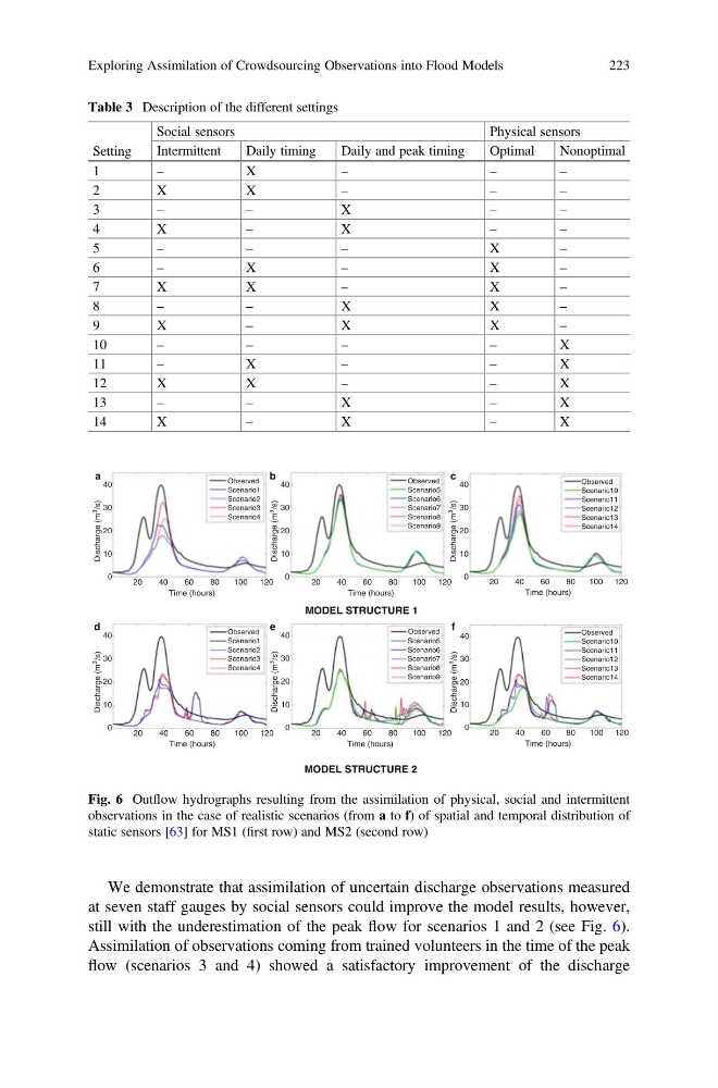
We demonstrate that assimilation of uncertain discharge observations measured
at seven staff gauges by social sensors could improve the model results, however,
still with the underestimation of the peak flow for scenarios 1 and 2 (see Fig. 6).
Assimilation of observations coming from trained volunteers in the time of the peak
flow (scenarios 3 and 4) showed a satisfactory improvement of the discharge
Table 3 Description of the different settings
Setting
Social sensors
Physical sensors
Intermittent
Daily timing
Daily and peak timing
Optimal
Nonoptimal
1
–
X
–
–
–
2
X
X
–
–
–
3
–
–
X
–
–
4
X
–
X
–
–
5
–
–
–
X
–
6
–
X
–
X
–
7
X
X
–
X
–
8
–
–
X
X
–
9
X
–
X
X
–
10
–
–
–
–
X
11
–
X
–
–
X
12
X
X
–
–
X
13
–
–
X
–
X
14
X
–
X
–
X
40
30
20
10
0
Time (hours)
Observed
Scenario1
Scenario2
Scenario3
Scenario4
Observed
Scenario5
Scenario6
Scenario7
Scenario8
Scenario9
Observed
Scenario10
Scenario11
Scenario12
Scenario13
Scenario14
Observed
Scenario1
Scenario2
Scenario3
Scenario4
Observed
Scenario5
Scenario6
Scenario7
Scenario8
Scenario9
Observed
Scenario10
Scenario11
Scenario12
Scenario13
Scenario14
Discharge (m 3
/s)
40
30
20
10
0
Discharge (m 3
/s)
20
40
60
80
100 120
Time (hours)
20
40
60
80
100 120
40
30
20
10
0
Discharge (m 3
/s)
Discharge (m 3
/s)
Time (hours)
20
40
60
80
100 120
40
30
20
10
0
Time (hours)
20
40
60
80
100 120
40
30
20
10
0
Time (hours)
MODEL STRUCTURE 1
a
b
c
d
e
f
MODEL STRUCTURE 2
Discharge (m 3
/s)
20
40
60
80
100 120
40
30
20
10
0
Time (hours)
Discharge (m 3
/s)
20
40
60
80
100 120
Fig. 6 Outflow hydrographs resulting from the assimilation of physical, social and intermittent
observations in the case of realistic scenarios (from a to f) of spatial and temporal distribution of
static sensors [63] for MS1 (first row) and MS2 (second row)
Exploring Assimilation of Crowdsourcing Observations into Flood Models
223