

4.3 Synthetic Flow Observations
Synthetic flow observations are used because of the lack of distributed crowdsourced
observations at the time of this study within the considered case study [62]. Such
synthetic observations are generated by two different approaches for the two catchments. On the one hand, for the Brue catchment, the approach used to generate the
synthetic values of river flow is very similar to the one used by Weerts and El Serafy
[90], in which the model forcing is perturbed by means of a time series normally
distributed with zero mean and given standard deviation.
On the other hand, for the Bacchiglione catchment, the observed time series of
precipitation are used as input for the hydrological models of the sub-catchments and
inter-catchments to generate synthetic discharges and then propagate them with the
hydraulic model down to the outlet point of the catchment. In this way, the synthetic
WL values at the outlet of the sub-catchments or inter-catchments and at each spatial
discretization of the six reaches of the Bacchiglione River are estimated and assumed
as observed variables in the assimilation process.
4.4 Estimation of the Observational Error
The correct estimation of the model and observational error is crucial for
implementing data assimilation methods. Few studies in the past have addressed
this issue (e.g. [95]), but further research is needed. For this reason, we adopted a
simplified approach to quantify observational errors. Here, the covariance matrix
R is assessed using the approach described in Weerts and El Serafy [90], Rakovec
et al. [43] and Mazzoleni [63]:
R t ¼ α t ∙ Q
synth
t
À
Á 2
ð10Þ
where α is a variable related to the accuracy level (i.e. degree to which the measurement is correct overall) of the flow measurement and Q
synth is the synthetic flow
observation. In the case of CS observations, accuracy levels vary temporally and
spatially.
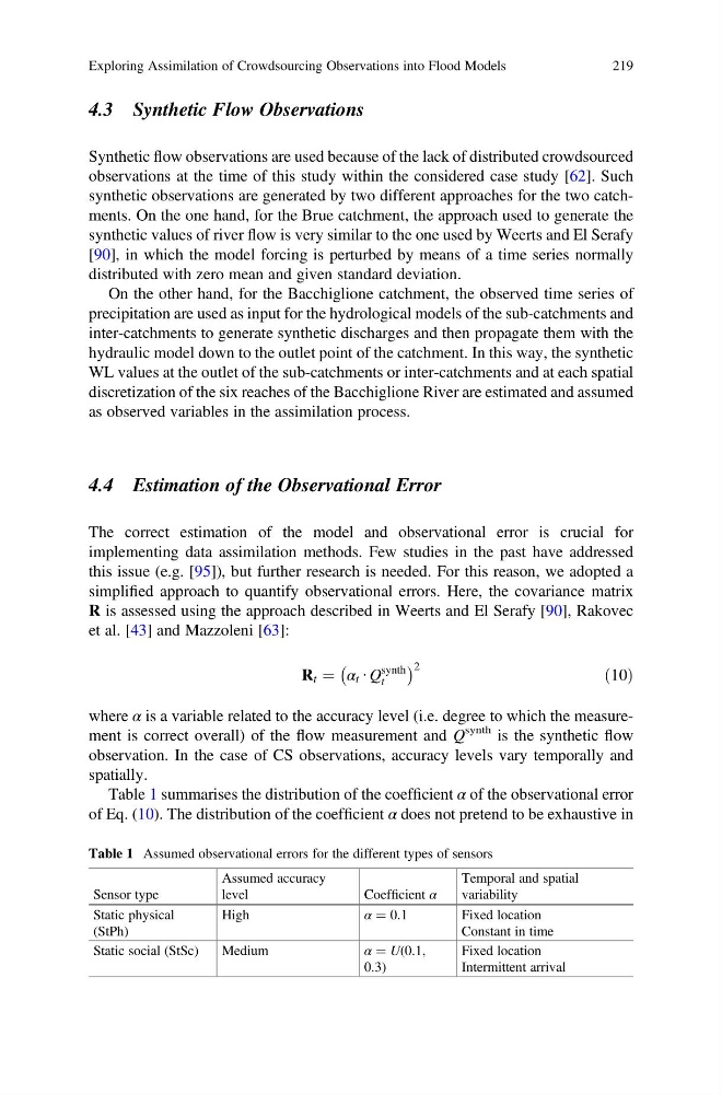
Table 1 summarises the distribution of the coefficient α of the observational error
of Eq. (10). The distribution of the coefficient α does not pretend to be exhaustive in
Table 1 Assumed observational errors for the different types of sensors
Sensor type
Assumed accuracy
level
Coefficient α
Temporal and spatial
variability
Static physical
(StPh)
High
α ¼ 0.1
Fixed location
Constant in time
Static social (StSc)
Medium
α ¼ U(0.1,
0.3)
Fixed location
Intermittent arrival
Exploring Assimilation of Crowdsourcing Observations into Flood Models
219
Synthetic flow observations are used because of the lack of distributed crowdsourced
observations at the time of this study within the considered case study [62]. Such
synthetic observations are generated by two different approaches for the two catchments. On the one hand, for the Brue catchment, the approach used to generate the
synthetic values of river flow is very similar to the one used by Weerts and El Serafy
[90], in which the model forcing is perturbed by means of a time series normally
distributed with zero mean and given standard deviation.
On the other hand, for the Bacchiglione catchment, the observed time series of
precipitation are used as input for the hydrological models of the sub-catchments and
inter-catchments to generate synthetic discharges and then propagate them with the
hydraulic model down to the outlet point of the catchment. In this way, the synthetic
WL values at the outlet of the sub-catchments or inter-catchments and at each spatial
discretization of the six reaches of the Bacchiglione River are estimated and assumed
as observed variables in the assimilation process.
4.4 Estimation of the Observational Error
The correct estimation of the model and observational error is crucial for
implementing data assimilation methods. Few studies in the past have addressed
this issue (e.g. [95]), but further research is needed. For this reason, we adopted a
simplified approach to quantify observational errors. Here, the covariance matrix
R is assessed using the approach described in Weerts and El Serafy [90], Rakovec
et al. [43] and Mazzoleni [63]:
R t ¼ α t ∙ Q
synth
t
À
Á 2
ð10Þ
where α is a variable related to the accuracy level (i.e. degree to which the measurement is correct overall) of the flow measurement and Q
synth is the synthetic flow
observation. In the case of CS observations, accuracy levels vary temporally and
spatially.
Table 1 summarises the distribution of the coefficient α of the observational error
of Eq. (10). The distribution of the coefficient α does not pretend to be exhaustive in
Table 1 Assumed observational errors for the different types of sensors
Sensor type
Assumed accuracy
level
Coefficient α
Temporal and spatial
variability
Static physical
(StPh)
High
α ¼ 0.1
Fixed location
Constant in time
Static social (StSc)
Medium
α ¼ U(0.1,
0.3)
Fixed location
Intermittent arrival
Exploring Assimilation of Crowdsourcing Observations into Flood Models
219