

284
I. Thiaw et al.
2.3 Methods
In this study, two hydrological models of RS Minerve (GR4J and SAC-SMA) were
compared. The model that best reproduced the hydrographs observed during the
calibration (1975–1992) and validation (1998–2003) phases were used to reconstruct
flow data that was missing for the Diarha over three periods (1961–1974; 1993–1997
and 2004–2012). This enabled consideration of a continuous period of discharges
from 1961 to 2012. In addition, the same model was used to project future flows
(horizon 2050) to anticipate the impact of climate change on surface water resources
of the Diarha catchment. CORDEX simulations produced climate outputs that were
subject to three RCM (IPSL-CM5A-LR, INM-CM4, and GFDL-ESM2G). In addition, characteristic high (DCC) and low (DCE) flow rates were applied to projected
climate scenarios through 2050.
2.3.1 Structure of Hydrological Models
GR4J Hydrological Model
The GR4J model (Perrin et al. 2003) is based on two reservoirs (production and
routing) and two unitary hydrographs (UH1 and UH2). The model simulates flows
through the production and transfer functions (Fig. 4). It first neutralizes equivalent
daily rainfall (Peq) by potential daily evapotranspiration to determine net rain (Pn)
and net evapotranspiration (En) (Garcia Hernandez et al. 2018):
Pn = Peq−E T P
En = 0 Si P ≥ E T P
Pn = 0 Si P > E T P
En = E T P − Peq
(1)
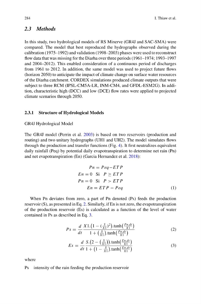
When Pn deviates from zero, a part of Pn denoted (Ps) feeds the production
reservoir (S), as presented in Eq. 2. Similarly, if En is not zero, the evapotranspiration
of the production reservoir (Es) is calculated as a function of the level of water
contained in Ps as described in Eq. 3.
Ps =
d
dt
X 1.
1 − (
S
X 1
)
2
.tanh
Pn.dt
X 1
1 +
S
X 1
.tanh
Pn.dt
X 1
(2)
Es =
d
dt
S.
2 −
S
X 1
.tanh
En.dt
X 1
1 +
1 −
S
X 1
.tanh
En.dt
X 1
(3)
where
Ps intensity of the rain feeding the production reservoir
I. Thiaw et al.
2.3 Methods
In this study, two hydrological models of RS Minerve (GR4J and SAC-SMA) were
compared. The model that best reproduced the hydrographs observed during the
calibration (1975–1992) and validation (1998–2003) phases were used to reconstruct
flow data that was missing for the Diarha over three periods (1961–1974; 1993–1997
and 2004–2012). This enabled consideration of a continuous period of discharges
from 1961 to 2012. In addition, the same model was used to project future flows
(horizon 2050) to anticipate the impact of climate change on surface water resources
of the Diarha catchment. CORDEX simulations produced climate outputs that were
subject to three RCM (IPSL-CM5A-LR, INM-CM4, and GFDL-ESM2G). In addition, characteristic high (DCC) and low (DCE) flow rates were applied to projected
climate scenarios through 2050.
2.3.1 Structure of Hydrological Models
GR4J Hydrological Model
The GR4J model (Perrin et al. 2003) is based on two reservoirs (production and
routing) and two unitary hydrographs (UH1 and UH2). The model simulates flows
through the production and transfer functions (Fig. 4). It first neutralizes equivalent
daily rainfall (Peq) by potential daily evapotranspiration to determine net rain (Pn)
and net evapotranspiration (En) (Garcia Hernandez et al. 2018):
Pn = Peq−E T P
En = 0 Si P ≥ E T P
Pn = 0 Si P > E T P
En = E T P − Peq
(1)
When Pn deviates from zero, a part of Pn denoted (Ps) feeds the production
reservoir (S), as presented in Eq. 2. Similarly, if En is not zero, the evapotranspiration
of the production reservoir (Es) is calculated as a function of the level of water
contained in Ps as described in Eq. 3.
Ps =
d
dt
X 1.
1 − (
S
X 1
)
2
.tanh
Pn.dt
X 1
1 +
S
X 1
.tanh
Pn.dt
X 1
(2)
Es =
d
dt
S.
2 −
S
X 1
.tanh
En.dt
X 1
1 +
1 −
S
X 1
.tanh
En.dt
X 1
(3)
where
Ps intensity of the rain feeding the production reservoir