

Example 15.6
Again analysing the same problem as outlined in Example 15.4, the decision-makers
analyse the same six criteria, this time using the pairwise comparison method.
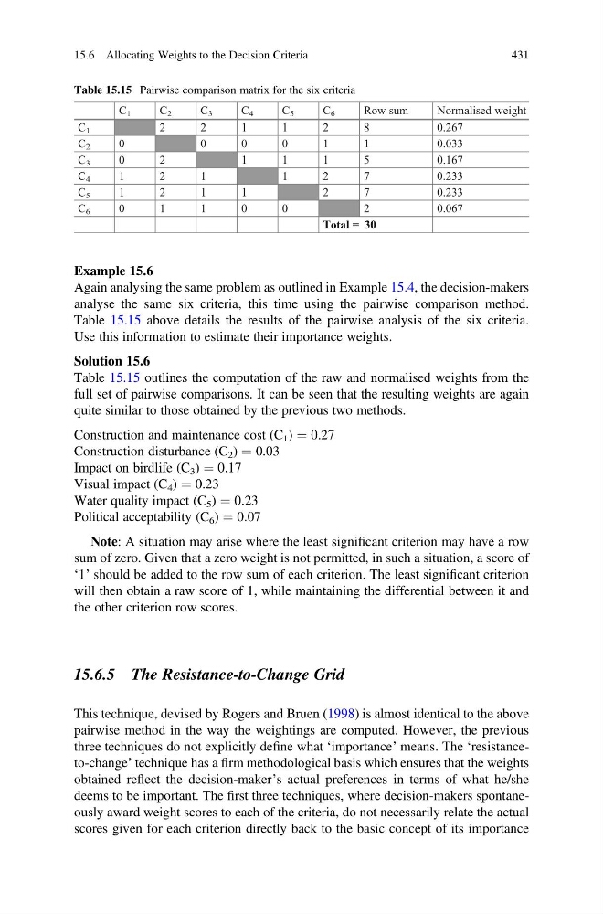
Table 15.15 above details the results of the pairwise analysis of the six criteria.
Use this information to estimate their importance weights.
Solution 15.6
Table 15.15 outlines the computation of the raw and normalised weights from the
full set of pairwise comparisons. It can be seen that the resulting weights are again
quite similar to those obtained by the previous two methods.
Construction and maintenance cost (C 1 ) ¼ 0.27
Construction disturbance (C 2 ) ¼ 0.03
Impact on birdlife (C 3 ) ¼ 0.17
Visual impact (C 4 ) ¼ 0.23
Water quality impact (C 5 ) ¼ 0.23
Political acceptability (C 6 ) ¼ 0.07
Note: A situation may arise where the least significant criterion may have a row
sum of zero. Given that a zero weight is not permitted, in such a situation, a score of
‘1’ should be added to the row sum of each criterion. The least significant criterion
will then obtain a raw score of 1, while maintaining the differential between it and
the other criterion row scores.
15.6.5 The Resistance-to-Change Grid
This technique, devised by Rogers and Bruen (1998) is almost identical to the above
pairwise method in the way the weightings are computed. However, the previous
three techniques do not explicitly define what ‘importance’ means. The ‘resistanceto-change’ technique has a firm methodological basis which ensures that the weights
obtained reflect the decision-maker’s actual preferences in terms of what he/she
deems to be important. The first three techniques, where decision-makers spontaneously award weight scores to each of the criteria, do not necessarily relate the actual
scores given for each criterion directly back to the basic concept of its importance
Table 15.15 Pairwise comparison matrix for the six criteria
C 1
C 2
C 3
C 4
C 5
C 6
Row sum
Normalised weight
C 1
2
2
1
1
2
8
0.267
C 2
0
0
0
0
1
1
0.033
C 3
0
2
1
1
1
5
0.167
C 4
1
2
1
1
2
7
0.233
C 5
1
2
1
1
2
7
0.233
C 6
0
1
1
0
0
2
0.067
Total = 30
15.6 Allocating Weights to the Decision Criteria
431
Again analysing the same problem as outlined in Example 15.4, the decision-makers
analyse the same six criteria, this time using the pairwise comparison method.
Table 15.15 above details the results of the pairwise analysis of the six criteria.
Use this information to estimate their importance weights.
Solution 15.6
Table 15.15 outlines the computation of the raw and normalised weights from the
full set of pairwise comparisons. It can be seen that the resulting weights are again
quite similar to those obtained by the previous two methods.
Construction and maintenance cost (C 1 ) ¼ 0.27
Construction disturbance (C 2 ) ¼ 0.03
Impact on birdlife (C 3 ) ¼ 0.17
Visual impact (C 4 ) ¼ 0.23
Water quality impact (C 5 ) ¼ 0.23
Political acceptability (C 6 ) ¼ 0.07
Note: A situation may arise where the least significant criterion may have a row
sum of zero. Given that a zero weight is not permitted, in such a situation, a score of
‘1’ should be added to the row sum of each criterion. The least significant criterion
will then obtain a raw score of 1, while maintaining the differential between it and
the other criterion row scores.
15.6.5 The Resistance-to-Change Grid
This technique, devised by Rogers and Bruen (1998) is almost identical to the above
pairwise method in the way the weightings are computed. However, the previous
three techniques do not explicitly define what ‘importance’ means. The ‘resistanceto-change’ technique has a firm methodological basis which ensures that the weights
obtained reflect the decision-maker’s actual preferences in terms of what he/she
deems to be important. The first three techniques, where decision-makers spontaneously award weight scores to each of the criteria, do not necessarily relate the actual
scores given for each criterion directly back to the basic concept of its importance
Table 15.15 Pairwise comparison matrix for the six criteria
C 1
C 2
C 3
C 4
C 5
C 6
Row sum
Normalised weight
C 1
2
2
1
1
2
8
0.267
C 2
0
0
0
0
1
1
0.033
C 3
0
2
1
1
1
5
0.167
C 4
1
2
1
1
2
7
0.233
C 5
1
2
1
1
2
7
0.233
C 6
0
1
1
0
0
2
0.067
Total = 30
15.6 Allocating Weights to the Decision Criteria
431