

K FODL ¼ AK A exp ½Àj2πf T FOS þ T 1FOS
ð
Þ
þBK B exp Àj2πf T FOS þ T 2FOS
ð
Þ
½
þ CK C exp Àj2πf T FOS þ T 3FOS
ð
Þ
½
þÁ Á Á þ NK N exp Àj2πf T FOS þ T NFOS
ð
Þ
½
,
ð6:63Þ
where T FOS + T 1FOS , T FOS + T 2FOS , T FOS + T 3FOS , T FOS + T NFOS are the light delays,
relatively, in first, second, third, and Nth optical channels. A Á K A , B Á K B , C Á K C , . . .
are products of the excitation coefficients of optical fibers by the modules of their
transfer functions, relatively, of optical fibers 1, 2, 3, 4, . . ., N.
6.5.10 Utilization of Differential and Combined FOS
to Suppress the Resonance
Differences in delays between the “adjacent” channels of optical channels should
satisfy the condition F T 2FOS À T 1FOS
ð
Þ ¼
1
N . Minima of K FODL modules should
correspond to the frequency values, which are not included into the generation of
OEO MZ. Figure 6.22 shows AFC of differential and combined RF FODL with two,
three, and four optical fibers of different geometrical length, which are used in OEO
for suppression of the adjacent (from the fundamental harmonic) types of oscillations, which are not attracted into generation.
From Fig. 6.22, we see that at differential RF FODL with two optical fibers, the
first minimum of AFC satisfies to the condition F(T 2FOS À T 1FOS ) ¼ 1/2, further, the
position of adjacent next minimum is defined as F T 2FOS À T 1FOS
ð
Þ ¼
1
2 þ 1.
The deeper suppression of the spurious noise harmonics can be achieved at
application of RF FODL consisting of three and more fibers with different length
(Fig. 6.22). We should note that the growth of optical channel number with utilization of Y-couplers leads to the increase of total losses in RF FODL and to decrease of
its transfer function |K FODL | and therefore it restricts its usage.
P OEO
P OEO
P 0L
K 2
ΓPN
K 2
ΓPN
K 2
ΓPN
P 0L
K 2
ΓPN
(b)
P 0L
Y 00
laser power,
(a)
P 0L
Y 00
laser power,
P
OEO
K 2
ΓPN ,
P
0L
K 2
ΓPN
,
0.005
5
1 5
10
20
0.010
0.050
0.100
0.500
1
P
OEO
K 2
ΓPN ,
P
0L
K 2
ΓPN
,
0.005
0.01
0.05 0.10
0.50 1
5 10
0.010
0.050
0.100
0.500
1
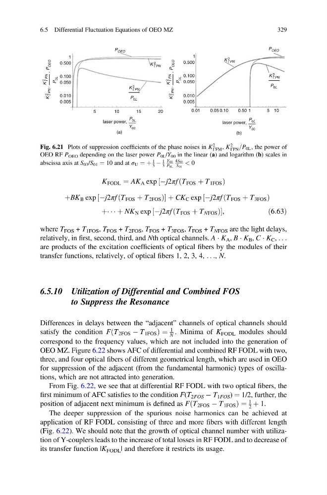
Fig. 6.21 Plots of suppression coefficients of the phase noises in K
2
ΓFM , K
2
ΓPN =P 0L , the power of
OEO RF P OEO depending on the laser power P 0L /Y 00 in the linear (а) and logarithm (b) scales in
abscissa axis at S 03 /S 01 ¼ 10 and at σ U ¼ þ
1
3 À
1
3
Y00
P0L
4S03
S01 < 0
6.5 Differential Fluctuation Equations of OEO MZ
329
ð
Þ
þBK B exp Àj2πf T FOS þ T 2FOS
ð
Þ
½
þ CK C exp Àj2πf T FOS þ T 3FOS
ð
Þ
½
þÁ Á Á þ NK N exp Àj2πf T FOS þ T NFOS
ð
Þ
½
,
ð6:63Þ
where T FOS + T 1FOS , T FOS + T 2FOS , T FOS + T 3FOS , T FOS + T NFOS are the light delays,
relatively, in first, second, third, and Nth optical channels. A Á K A , B Á K B , C Á K C , . . .
are products of the excitation coefficients of optical fibers by the modules of their
transfer functions, relatively, of optical fibers 1, 2, 3, 4, . . ., N.
6.5.10 Utilization of Differential and Combined FOS
to Suppress the Resonance
Differences in delays between the “adjacent” channels of optical channels should
satisfy the condition F T 2FOS À T 1FOS
ð
Þ ¼
1
N . Minima of K FODL modules should
correspond to the frequency values, which are not included into the generation of
OEO MZ. Figure 6.22 shows AFC of differential and combined RF FODL with two,
three, and four optical fibers of different geometrical length, which are used in OEO
for suppression of the adjacent (from the fundamental harmonic) types of oscillations, which are not attracted into generation.
From Fig. 6.22, we see that at differential RF FODL with two optical fibers, the
first minimum of AFC satisfies to the condition F(T 2FOS À T 1FOS ) ¼ 1/2, further, the
position of adjacent next minimum is defined as F T 2FOS À T 1FOS
ð
Þ ¼
1
2 þ 1.
The deeper suppression of the spurious noise harmonics can be achieved at
application of RF FODL consisting of three and more fibers with different length
(Fig. 6.22). We should note that the growth of optical channel number with utilization of Y-couplers leads to the increase of total losses in RF FODL and to decrease of
its transfer function |K FODL | and therefore it restricts its usage.
P OEO
P OEO
P 0L
K 2
ΓPN
K 2
ΓPN
K 2
ΓPN
P 0L
K 2
ΓPN
(b)
P 0L
Y 00
laser power,
(a)
P 0L
Y 00
laser power,
P
OEO
K 2
ΓPN ,
P
0L
K 2
ΓPN
,
0.005
5
1 5
10
20
0.010
0.050
0.100
0.500
1
P
OEO
K 2
ΓPN ,
P
0L
K 2
ΓPN
,
0.005
0.01
0.05 0.10
0.50 1
5 10
0.010
0.050
0.100
0.500
1
Fig. 6.21 Plots of suppression coefficients of the phase noises in K
2
ΓFM , K
2
ΓPN =P 0L , the power of
OEO RF P OEO depending on the laser power P 0L /Y 00 in the linear (а) and logarithm (b) scales in
abscissa axis at S 03 /S 01 ¼ 10 and at σ U ¼ þ
1
3 À
1
3
Y00
P0L
4S03
S01 < 0
6.5 Differential Fluctuation Equations of OEO MZ
329