

R MZ u,t,tþτ
ð
Þ
¼
τ
j j> ΔT M
j
j!
1
2
exp ÀΔν L Á2 ΔT M
j
j
ð
Þ 1þ cos 2Á2πν L τ
ð
Þ
½
,
τ
j j ΔT M
j
j!
1
2
exp ÀΔν L Á2 τ
j j
ð
Þ þ exp ÀΔν L Á 4 ΔT M
j
jÀ2 τ
j j
ð
Þ
ð
Þ Á cos 2Á2πν L τ
ð
Þ
½
:
8
> <
> :
ð5:93Þ
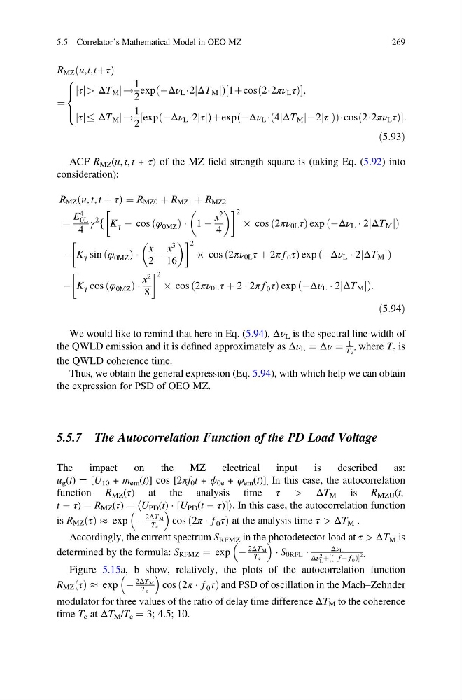
ACF R MZ (u, t, t + τ) of the MZ field strength square is (taking Eq. (5.92) into
consideration):
R MZ u, t, t þ τ
ð
Þ¼R MZ0 þ R MZ1 þ R MZ2
¼
E
4
0L
4
γ
2
f K γ À cos φ 0MZ
ð
ÞÁ 1 À
x
2
4
! 2
 cos 2πν 0L τ
ð
Þexp ÀΔν L Á 2 ΔT M
j
j
ð
Þ
À K γ sin φ 0MZ
ð
ÞÁ
x
2
À
x
3
16
! 2
 cos 2πν 0L τ þ 2π f 0 τ
ð
Þ exp ÀΔν L Á 2 ΔT M
j
j
ð
Þ
À K γ cos φ 0MZ
ð
ÞÁ
x
2
8
! 2
 cos 2πν 0L τ þ 2 Á 2π f 0 τ
ð
Þ exp ÀΔν L Á 2 ΔT M
j
j
ð
Þ :
ð5:94Þ
We would like to remind that here in Eq. (5.94), Δν L is the spectral line width of
the QWLD emission and it is defined approximately as Δν L ¼ Δν ¼
1
T c
, where T c is
the QWLD coherence time.
Thus, we obtain the general expression (Eq. 5.94), with which help we can obtain
the expression for PSD of OEO MZ.
5.5.7 The Autocorrelation Function of the PD Load Voltage
The
impact
on
the
MZ
electrical
input
is
described
as:
u g (t) ¼ [U 10 + m em (t)] cos [2πf 0 t + ϕ 0e + φ em (t)] . In this case, the autocorrelation
function R MZ (τ) at the analysis time τ > ΔT M is R MZU (t,
t À τ) ¼ R MZ (τ) ¼ hU PD (t) Á [U PD (t À τ)]i. In this case, the autocorrelation function
is R MZ τ
ð Þ % exp À
2ΔT M
T c
cos 2π Á f 0 τ
ð
Þat the analysis time τ > ΔT M .
Accordingly, the current spectrum S RFMZ in the photodetector load at τ > ΔT M is
determined by the formula: S RFMZ ¼ exp À
2ΔT M
T c
Á S 0RFL Á
Δν L
Δν 2
L
þ f À f 0
ð
Þ
½
2 .
Figure 5.15a, b show, relatively, the plots of the autocorrelation function
R MZ τ
ð Þ % exp À
2ΔT M
T c
cos 2π Á f 0 τ
ð
Þand PSD of oscillation in the Mach–Zehnder
modulator for three values of the ratio of delay time difference ΔT M to the coherence
time T c at ΔT M /T c ¼ 3; 4.5; 10.
5.5 Correlator’s Mathematical Model in OEO MZ
269
ð
Þ
¼
τ
j j> ΔT M
j
j!
1
2
exp ÀΔν L Á2 ΔT M
j
j
ð
Þ 1þ cos 2Á2πν L τ
ð
Þ
½
,
τ
j j ΔT M
j
j!
1
2
exp ÀΔν L Á2 τ
j j
ð
Þ þ exp ÀΔν L Á 4 ΔT M
j
jÀ2 τ
j j
ð
Þ
ð
Þ Á cos 2Á2πν L τ
ð
Þ
½
:
8
> <
> :
ð5:93Þ
ACF R MZ (u, t, t + τ) of the MZ field strength square is (taking Eq. (5.92) into
consideration):
R MZ u, t, t þ τ
ð
Þ¼R MZ0 þ R MZ1 þ R MZ2
¼
E
4
0L
4
γ
2
f K γ À cos φ 0MZ
ð
ÞÁ 1 À
x
2
4
! 2
 cos 2πν 0L τ
ð
Þexp ÀΔν L Á 2 ΔT M
j
j
ð
Þ
À K γ sin φ 0MZ
ð
ÞÁ
x
2
À
x
3
16
! 2
 cos 2πν 0L τ þ 2π f 0 τ
ð
Þ exp ÀΔν L Á 2 ΔT M
j
j
ð
Þ
À K γ cos φ 0MZ
ð
ÞÁ
x
2
8
! 2
 cos 2πν 0L τ þ 2 Á 2π f 0 τ
ð
Þ exp ÀΔν L Á 2 ΔT M
j
j
ð
Þ :
ð5:94Þ
We would like to remind that here in Eq. (5.94), Δν L is the spectral line width of
the QWLD emission and it is defined approximately as Δν L ¼ Δν ¼
1
T c
, where T c is
the QWLD coherence time.
Thus, we obtain the general expression (Eq. 5.94), with which help we can obtain
the expression for PSD of OEO MZ.
5.5.7 The Autocorrelation Function of the PD Load Voltage
The
impact
on
the
MZ
electrical
input
is
described
as:
u g (t) ¼ [U 10 + m em (t)] cos [2πf 0 t + ϕ 0e + φ em (t)] . In this case, the autocorrelation
function R MZ (τ) at the analysis time τ > ΔT M is R MZU (t,
t À τ) ¼ R MZ (τ) ¼ hU PD (t) Á [U PD (t À τ)]i. In this case, the autocorrelation function
is R MZ τ
ð Þ % exp À
2ΔT M
T c
cos 2π Á f 0 τ
ð
Þat the analysis time τ > ΔT M .
Accordingly, the current spectrum S RFMZ in the photodetector load at τ > ΔT M is
determined by the formula: S RFMZ ¼ exp À
2ΔT M
T c
Á S 0RFL Á
Δν L
Δν 2
L
þ f À f 0
ð
Þ
½
2 .
Figure 5.15a, b show, relatively, the plots of the autocorrelation function
R MZ τ
ð Þ % exp À
2ΔT M
T c
cos 2π Á f 0 τ
ð
Þand PSD of oscillation in the Mach–Zehnder
modulator for three values of the ratio of delay time difference ΔT M to the coherence
time T c at ΔT M /T c ¼ 3; 4.5; 10.
5.5 Correlator’s Mathematical Model in OEO MZ
269