

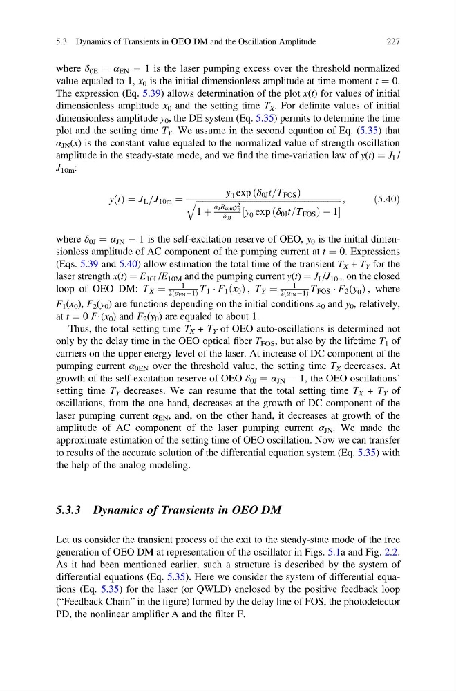
where δ 0E ¼ α EN À 1 is the laser pumping excess over the threshold normalized
value equaled to 1, x 0 is the initial dimensionless amplitude at time moment t ¼ 0.
The expression (Eq. 5.39) allows determination of the plot x(t) for values of initial
dimensionless amplitude x 0 and the setting time T X . For definite values of initial
dimensionless amplitude y 0 , the DE system (Eq. 5.35) permits to determine the time
plot and the setting time T Y . We assume in the second equation of Eq. (5.35) that
α JN (x) is the constant value equaled to the normalized value of strength oscillation
amplitude in the steady-state mode, and we find the time-variation law of y(t) ¼ J L /
J 10m :
y t
ð Þ ¼ J L =J 10m ¼
y 0 exp δ 0J t=T FOS
ð
Þ
ffiffiffiffiffiffiffiffiffiffiffiffiffiffiffiffiffiffiffiffiffiffiffiffiffiffiffiffiffiffiffiffiffiffiffiffiffiffiffiffiffiffiffiffiffiffiffiffiffiffiffiffiffiffiffiffiffiffiffiffiffiffiffiffiffiffiffi ffi
1 þ
α J R cont y 2
0
δ 0J
y 0 exp δ 0J t=T FOS
ð
ÞÀ1
½
q
,
ð5:40Þ
where δ 0J ¼ α JN À 1 is the self-excitation reserve of OEO, y 0 is the initial dimensionless amplitude of AC component of the pumping current at t ¼ 0. Expressions
(Eqs. 5.39 and 5.40) allow estimation the total time of the transient T X + T Y for the
laser strength x(t) ¼ E 10L /E 10M and the pumping current y(t) ¼ J L /J 10m on the closed
loop of OEO DM: T X ¼
1
2 α EN À1
ð
Þ T 1 Á F 1 x 0
ð Þ , T Y ¼
1
2 α JN À1
ð
Þ T FOS Á F 2 y 0
ð Þ , where
F 1 (x 0 ), F 2 (y 0 ) are functions depending on the initial conditions x 0 and y 0 , relatively,
at t ¼ 0 F 1 (x 0 ) and F 2 (y 0 ) are equaled to about 1.
Thus, the total setting time T X + T Y of OEO auto-oscillations is determined not
only by the delay time in the OEO optical fiber T FOS , but also by the lifetime T 1 of
carriers on the upper energy level of the laser. At increase of DC component of the
pumping current α 0EN over the threshold value, the setting time T X decreases. At
growth of the self-excitation reserve of OEO δ 0J ¼ α JN À 1, the OEO oscillations’
setting time T Y decreases. We can resume that the total setting time T X + T Y of
oscillations, from the one hand, decreases at the growth of DC component of the
laser pumping current α EN , and, on the other hand, it decreases at growth of the
amplitude of AC component of the laser pumping current α JN . We made the
approximate estimation of the setting time of OEO oscillation. Now we can transfer
to results of the accurate solution of the differential equation system (Eq. 5.35) with
the help of the analog modeling.
5.3.3 Dynamics of Transients in OEO DM
Let us consider the transient process of the exit to the steady-state mode of the free
generation of OEO DM at representation of the oscillator in Figs. 5.1a and Fig. 2.2.
As it had been mentioned earlier, such a structure is described by the system of
differential equations (Eq. 5.35). Here we consider the system of differential equations (Eq. 5.35) for the laser (or QWLD) enclosed by the positive feedback loop
(“Feedback Chain” in the figure) formed by the delay line of FOS, the photodetector
PD, the nonlinear amplifier A and the filter F.
5.3 Dynamics of Transients in ОЕО DM and the Oscillation Amplitude
227
value equaled to 1, x 0 is the initial dimensionless amplitude at time moment t ¼ 0.
The expression (Eq. 5.39) allows determination of the plot x(t) for values of initial
dimensionless amplitude x 0 and the setting time T X . For definite values of initial
dimensionless amplitude y 0 , the DE system (Eq. 5.35) permits to determine the time
plot and the setting time T Y . We assume in the second equation of Eq. (5.35) that
α JN (x) is the constant value equaled to the normalized value of strength oscillation
amplitude in the steady-state mode, and we find the time-variation law of y(t) ¼ J L /
J 10m :
y t
ð Þ ¼ J L =J 10m ¼
y 0 exp δ 0J t=T FOS
ð
Þ
ffiffiffiffiffiffiffiffiffiffiffiffiffiffiffiffiffiffiffiffiffiffiffiffiffiffiffiffiffiffiffiffiffiffiffiffiffiffiffiffiffiffiffiffiffiffiffiffiffiffiffiffiffiffiffiffiffiffiffiffiffiffiffiffiffiffiffi ffi
1 þ
α J R cont y 2
0
δ 0J
y 0 exp δ 0J t=T FOS
ð
ÞÀ1
½
q
,
ð5:40Þ
where δ 0J ¼ α JN À 1 is the self-excitation reserve of OEO, y 0 is the initial dimensionless amplitude of AC component of the pumping current at t ¼ 0. Expressions
(Eqs. 5.39 and 5.40) allow estimation the total time of the transient T X + T Y for the
laser strength x(t) ¼ E 10L /E 10M and the pumping current y(t) ¼ J L /J 10m on the closed
loop of OEO DM: T X ¼
1
2 α EN À1
ð
Þ T 1 Á F 1 x 0
ð Þ , T Y ¼
1
2 α JN À1
ð
Þ T FOS Á F 2 y 0
ð Þ , where
F 1 (x 0 ), F 2 (y 0 ) are functions depending on the initial conditions x 0 and y 0 , relatively,
at t ¼ 0 F 1 (x 0 ) and F 2 (y 0 ) are equaled to about 1.
Thus, the total setting time T X + T Y of OEO auto-oscillations is determined not
only by the delay time in the OEO optical fiber T FOS , but also by the lifetime T 1 of
carriers on the upper energy level of the laser. At increase of DC component of the
pumping current α 0EN over the threshold value, the setting time T X decreases. At
growth of the self-excitation reserve of OEO δ 0J ¼ α JN À 1, the OEO oscillations’
setting time T Y decreases. We can resume that the total setting time T X + T Y of
oscillations, from the one hand, decreases at the growth of DC component of the
laser pumping current α EN , and, on the other hand, it decreases at growth of the
amplitude of AC component of the laser pumping current α JN . We made the
approximate estimation of the setting time of OEO oscillation. Now we can transfer
to results of the accurate solution of the differential equation system (Eq. 5.35) with
the help of the analog modeling.
5.3.3 Dynamics of Transients in OEO DM
Let us consider the transient process of the exit to the steady-state mode of the free
generation of OEO DM at representation of the oscillator in Figs. 5.1a and Fig. 2.2.
As it had been mentioned earlier, such a structure is described by the system of
differential equations (Eq. 5.35). Here we consider the system of differential equations (Eq. 5.35) for the laser (or QWLD) enclosed by the positive feedback loop
(“Feedback Chain” in the figure) formed by the delay line of FOS, the photodetector
PD, the nonlinear amplifier A and the filter F.
5.3 Dynamics of Transients in ОЕО DM and the Oscillation Amplitude
227