

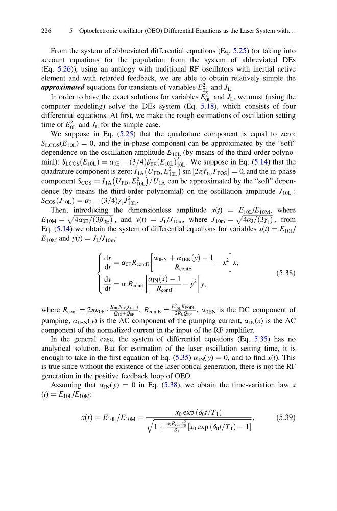
From the system of abbreviated differential equations (Eq. 5.25) (or taking into
account equations for the population from the system of abbreviated DEs
(Eq. 5.26)), using an analogy with traditional RF oscillators with inertial active
element and with retarded feedback, we are able to obtain relatively simple the
approximated equations for transients of variables E
2
0L and J L .
In order to have the exact solutions for variables E
2
0L and J L , we must (using the
computer modeling) solve the DEs system (Eq. 5.18), which consists of four
differential equations. At first, we make the rough estimations of oscillation setting
time of E
2
0L and J L for the simple case.
We suppose in Eq. (5.25) that the quadrature component is equal to zero:
S LCOS (E 10L ) ¼ 0, and the in-phase component can be approximated by the “soft”
dependence on the oscillation amplitude E 10L (by means of the third-order polynomial): S LCOS E 10L
ð
Þ¼ α 0E À 3=4
ð
Þβ 0E E 10L
ð
Þ
2
10L . We suppose in Eq. (5.14) that the
quadrature component is zero: I 1A U PD , E
2
10L
À
Á
sin 2π f 0e T FOS
½
¼0, and the in-phase
component S COS ¼ I 1A U PD , E
2
10L
À
Á =U 1A can be approximated by the “soft” dependence (by means the third-order polynomial) on the oscillation amplitude J 10L :
S COS J 10L
ð
Þ ¼ α J À 3=4
ð
Þγ J J
2
10L .
Then, introducing the dimensionless amplitude x(t) ¼ E 10L /E 10M , where
E 10M ¼
ffiffiffiffiffiffiffiffiffiffiffiffiffiffiffiffiffiffiffiffiffiffiffiffi
4α 0E = 3β 0E
ð
Þ
p
, and y(t) ¼ J L /J 10m , where J 10m ¼
ffiffiffiffiffiffiffiffiffiffiffiffiffiffiffiffiffiffiffi
4α J = 3γ J
ð Þ
p
, from
Eq. (5.14) we obtain the system of differential equations for variables x(t) ¼ E 10L /
E 10M and y(t) ¼ J L /J 10m :
dx
dt
¼ α 0E R contE
α 0EN þ α 1EN y
ð Þ À 1
R contE
À x
2
!
x,
dy
dt
¼ α J R contJ
α JN x
ð Þ À 1
R contJ
À y
2
!
y,
8
> > > <
> > > :
ð5:38Þ
where R cont ¼ 2πν 0F Á
K 0L N 0 J 10L
ð
Þ
Q 12 þQ 0F
, R contE ¼
E
2
10L K FODL
2R L Q EF
, α 0EN is the DC component of
pumping, α 1EN ( y) is the AC component of the pumping current, α JN (x) is the AC
component of the normalized current in the input of the RF amplifier.
In the general case, the system of differential equations (Eq. 5.35) has no
analytical solution. But for estimation of the laser oscillation setting time, it is
enough to take in the first equation of Eq. (5.35) α JN ( y) ¼ 0, and to find x(t). This
is true since without the existence of the laser optical generation, there is not the RF
generation in the positive feedback loop of OEO.
Assuming that α JN ( y) ¼ 0 in Eq. (5.38), we obtain the time-variation law x
(t) ¼ E 10L /E 10M :
x t
ð Þ ¼ E 10L =E 10M ¼
x 0 exp δ 0 t=T 1
ð
Þ
ffiffiffiffiffiffiffiffiffiffiffiffiffiffiffiffiffiffiffiffiffiffiffiffiffiffiffiffiffiffiffiffiffiffiffiffiffiffiffiffiffiffiffiffiffiffiffiffiffiffiffiffiffiffiffiffiffiffiffiffiffi ffi
1 þ
α J R cont x 2
0
δ 0
x 0 exp δ 0 t=T 1
ð
ÞÀ1
½
q
,
ð5:39Þ
226
5 Optoelectronic oscillator (OEO) Differential Equations as the Laser System with. . .
account equations for the population from the system of abbreviated DEs
(Eq. 5.26)), using an analogy with traditional RF oscillators with inertial active
element and with retarded feedback, we are able to obtain relatively simple the
approximated equations for transients of variables E
2
0L and J L .
In order to have the exact solutions for variables E
2
0L and J L , we must (using the
computer modeling) solve the DEs system (Eq. 5.18), which consists of four
differential equations. At first, we make the rough estimations of oscillation setting
time of E
2
0L and J L for the simple case.
We suppose in Eq. (5.25) that the quadrature component is equal to zero:
S LCOS (E 10L ) ¼ 0, and the in-phase component can be approximated by the “soft”
dependence on the oscillation amplitude E 10L (by means of the third-order polynomial): S LCOS E 10L
ð
Þ¼ α 0E À 3=4
ð
Þβ 0E E 10L
ð
Þ
2
10L . We suppose in Eq. (5.14) that the
quadrature component is zero: I 1A U PD , E
2
10L
À
Á
sin 2π f 0e T FOS
½
¼0, and the in-phase
component S COS ¼ I 1A U PD , E
2
10L
À
Á =U 1A can be approximated by the “soft” dependence (by means the third-order polynomial) on the oscillation amplitude J 10L :
S COS J 10L
ð
Þ ¼ α J À 3=4
ð
Þγ J J
2
10L .
Then, introducing the dimensionless amplitude x(t) ¼ E 10L /E 10M , where
E 10M ¼
ffiffiffiffiffiffiffiffiffiffiffiffiffiffiffiffiffiffiffiffiffiffiffiffi
4α 0E = 3β 0E
ð
Þ
p
, and y(t) ¼ J L /J 10m , where J 10m ¼
ffiffiffiffiffiffiffiffiffiffiffiffiffiffiffiffiffiffiffi
4α J = 3γ J
ð Þ
p
, from
Eq. (5.14) we obtain the system of differential equations for variables x(t) ¼ E 10L /
E 10M and y(t) ¼ J L /J 10m :
dx
dt
¼ α 0E R contE
α 0EN þ α 1EN y
ð Þ À 1
R contE
À x
2
!
x,
dy
dt
¼ α J R contJ
α JN x
ð Þ À 1
R contJ
À y
2
!
y,
8
> > > <
> > > :
ð5:38Þ
where R cont ¼ 2πν 0F Á
K 0L N 0 J 10L
ð
Þ
Q 12 þQ 0F
, R contE ¼
E
2
10L K FODL
2R L Q EF
, α 0EN is the DC component of
pumping, α 1EN ( y) is the AC component of the pumping current, α JN (x) is the AC
component of the normalized current in the input of the RF amplifier.
In the general case, the system of differential equations (Eq. 5.35) has no
analytical solution. But for estimation of the laser oscillation setting time, it is
enough to take in the first equation of Eq. (5.35) α JN ( y) ¼ 0, and to find x(t). This
is true since without the existence of the laser optical generation, there is not the RF
generation in the positive feedback loop of OEO.
Assuming that α JN ( y) ¼ 0 in Eq. (5.38), we obtain the time-variation law x
(t) ¼ E 10L /E 10M :
x t
ð Þ ¼ E 10L =E 10M ¼
x 0 exp δ 0 t=T 1
ð
Þ
ffiffiffiffiffiffiffiffiffiffiffiffiffiffiffiffiffiffiffiffiffiffiffiffiffiffiffiffiffiffiffiffiffiffiffiffiffiffiffiffiffiffiffiffiffiffiffiffiffiffiffiffiffiffiffiffiffiffiffiffiffi ffi
1 þ
α J R cont x 2
0
δ 0
x 0 exp δ 0 t=T 1
ð
ÞÀ1
½
q
,
ð5:39Þ
226
5 Optoelectronic oscillator (OEO) Differential Equations as the Laser System with. . .