

of A ¼ 0.0081 at parametric growth of the Q-factor. The further growth of A leads to
instability (the chaotic generation). At that, the amplitude values are defined ambiguously for the same values of the frequency. From an analysis of plots (Fig. 4.29b), we
state that branches of unstable and stable operation of the generator in the steady-state
mode come together from above and from below at growth of the A coefficient, which
achieves the critical magnitude of A ¼ 0.082 at parametric growth of the Q-factor. The
further growth of A leads to instability (the chaotic generation).
4.6.2.6 The Cubic Parametric Function of the Resonator Q-factor
Figure 4.30 shows the resonance characteristics at cubic function of the resonator Qfactor versus the field amplitude E
2
10n : (1/Q 0F ) + (1/Q 02 ) ¼ 0.0001 Á (1 À A Á (E 10n )
3 )
(Fig. 4.30a) and (1/Q 0F ) + (1/Q 02 ) ¼ 0.1 Á (1 + A Á (E 10n )
3 ) (Fig. 4.30b).
From the analysis of plots in Fig. 4.30a, we state that branches of unstable and
stable operation of the generator in the steady-state mode come close only from
above at growth of the A coefficient, which achieves the critical value of
A ¼ 0.0034 at parametric growth of the Q-factor. The further growth of A leads to
20
60
40
20
0
-20
1
2
2
1
3
10
0
3
1
2
2 3
1
-10
-20
-10 -5
0
a)
5 10
-3 -2-1 0 1 2 3
normalized optical
frequency
s = (v / v 0F ) (u.a.)
b)
normalized optical
frequency
s = (v / v 0F ) (u.a.)
amplitude
x =
E
10n
(s =
v /
v
0F
) (u.a.)
amplitude
x =
E
10n
(s =
v /
v
0F
) (u.a.)
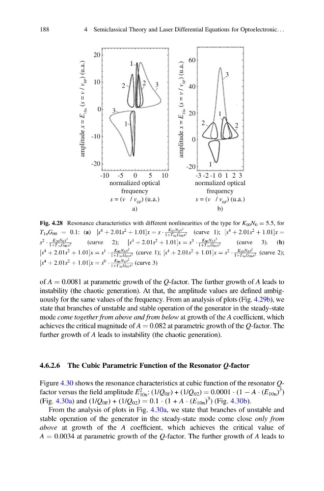
Fig. 4.28 Resonance characteristics with different nonlinearities of the type for K 00 N 0 ¼ 5.5, for
T 1n G 00 ¼ 0.1: (a) s
4 þ 2:01s
2 þ 1:01
½
x ¼ s Á
K00N0x
2
1þT1nG00x 2
(curve 1); s
4 þ 2:01s
2 þ 1:01
½
x ¼
s
2 Á
K00N0x
2
1þT1nG00x 2
(curve 2);
s
4 þ 2:01s
2 þ 1:01
½
x ¼ s
3 Á
K00N0x
2
1þT1nG00x 2
(curve 3). (b)
s
4 þ 2:01s
2 þ 1:01
½
x ¼ s
1 Á
K00N0x
2
1þT1nG00x 2 (curve 1); s
4 þ 2:01s
2 þ 1:01
½
x ¼ s
2 Á
K00N0x
2
1þT1nG00x 2 (curve 2);
s
4 þ 2:01s
2 þ 1:01
½
x ¼ s
0 Á
K00N0x
2
1þT1nG00x 2 (curve 3)
188
4 Semiclassical Theory and Laser Differential Equations for Optoelectronic. . .
instability (the chaotic generation). At that, the amplitude values are defined ambiguously for the same values of the frequency. From an analysis of plots (Fig. 4.29b), we
state that branches of unstable and stable operation of the generator in the steady-state
mode come together from above and from below at growth of the A coefficient, which
achieves the critical magnitude of A ¼ 0.082 at parametric growth of the Q-factor. The
further growth of A leads to instability (the chaotic generation).
4.6.2.6 The Cubic Parametric Function of the Resonator Q-factor
Figure 4.30 shows the resonance characteristics at cubic function of the resonator Qfactor versus the field amplitude E
2
10n : (1/Q 0F ) + (1/Q 02 ) ¼ 0.0001 Á (1 À A Á (E 10n )
3 )
(Fig. 4.30a) and (1/Q 0F ) + (1/Q 02 ) ¼ 0.1 Á (1 + A Á (E 10n )
3 ) (Fig. 4.30b).
From the analysis of plots in Fig. 4.30a, we state that branches of unstable and
stable operation of the generator in the steady-state mode come close only from
above at growth of the A coefficient, which achieves the critical value of
A ¼ 0.0034 at parametric growth of the Q-factor. The further growth of A leads to
20
60
40
20
0
-20
1
2
2
1
3
10
0
3
1
2
2 3
1
-10
-20
-10 -5
0
a)
5 10
-3 -2-1 0 1 2 3
normalized optical
frequency
s = (v / v 0F ) (u.a.)
b)
normalized optical
frequency
s = (v / v 0F ) (u.a.)
amplitude
x =
E
10n
(s =
v /
v
0F
) (u.a.)
amplitude
x =
E
10n
(s =
v /
v
0F
) (u.a.)
Fig. 4.28 Resonance characteristics with different nonlinearities of the type for K 00 N 0 ¼ 5.5, for
T 1n G 00 ¼ 0.1: (a) s
4 þ 2:01s
2 þ 1:01
½
x ¼ s Á
K00N0x
2
1þT1nG00x 2
(curve 1); s
4 þ 2:01s
2 þ 1:01
½
x ¼
s
2 Á
K00N0x
2
1þT1nG00x 2
(curve 2);
s
4 þ 2:01s
2 þ 1:01
½
x ¼ s
3 Á
K00N0x
2
1þT1nG00x 2
(curve 3). (b)
s
4 þ 2:01s
2 þ 1:01
½
x ¼ s
1 Á
K00N0x
2
1þT1nG00x 2 (curve 1); s
4 þ 2:01s
2 þ 1:01
½
x ¼ s
2 Á
K00N0x
2
1þT1nG00x 2 (curve 2);
s
4 þ 2:01s
2 þ 1:01
½
x ¼ s
0 Á
K00N0x
2
1þT1nG00x 2 (curve 3)
188
4 Semiclassical Theory and Laser Differential Equations for Optoelectronic. . .