

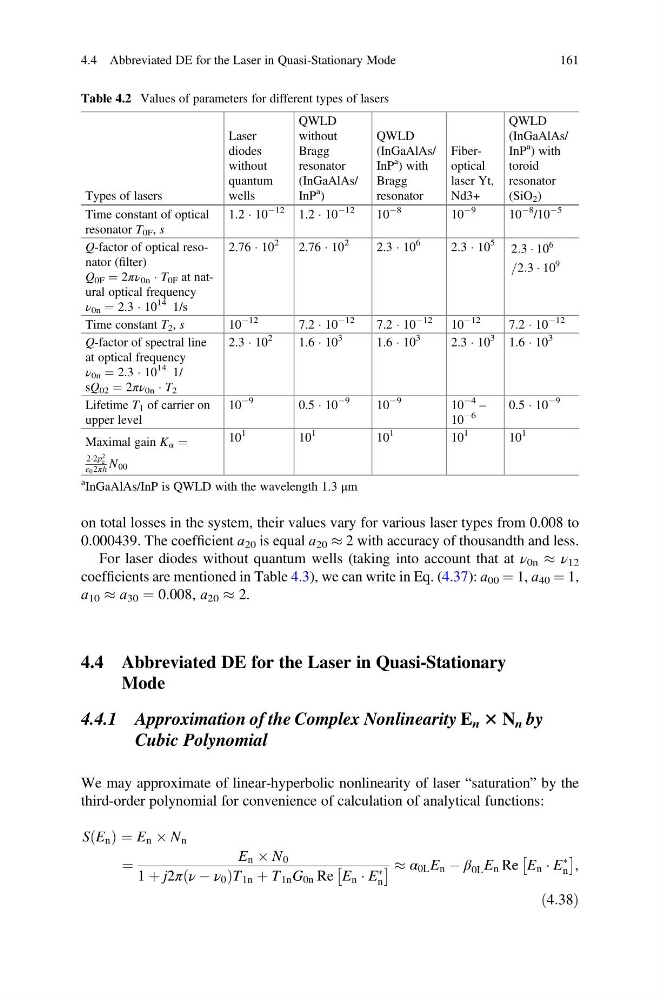
on total losses in the system, their values vary for various laser types from 0.008 to
0.000439. The coefficient а 20 is equal а 20 % 2 with accuracy of thousandth and less.
For laser diodes without quantum wells (taking into account that at ν 0n % ν 12
coefficients are mentioned in Table 4.3), we can write in Eq. (4.37): а 00 ¼ 1, а 40 ¼ 1,
а 10 % а 30 ¼ 0.008, а 20 % 2.
4.4 Abbreviated DE for the Laser in Quasi-Stationary
Mode
4.4.1 Approximation of the Complex Nonlinearity E n 3 N n by
Cubic Polynomial
We may approximate of linear-hyperbolic nonlinearity of laser “saturation” by the
third-order polynomial for convenience of calculation of analytical functions:
S E n
ð Þ ¼ E n  N n
¼
E n  N 0
1 þ j2π ν À ν 0
ð
ÞT 1n þ T 1n G 0n Re E n Á E
Ã
n
Â
Ã% α 0L E n À β 0L E n Re E n Á E
Ã
n
Â
Ã
,
ð4:38Þ
Table 4.2 Values of parameters for different types of lasers
Types of lasers
Laser
diodes
without
quantum
wells
QWLD
without
Bragg
resonator
(InGaAlAs/
InP
a )
QWLD
(InGaAlAs/
InP
a ) with
Bragg
resonator
Fiberoptical
laser Yt,
Nd3+
QWLD
(InGaAlAs/
InP
a ) with
toroid
resonator
(SiO 2 )
Time constant of optical
resonator T 0F , s
1.2 Á 10
À12
1.2 Á 10
À12
10
À8
10
À9
10
À8
/10
À5
Q-factor of optical resonator (filter)
Q 0F ¼ 2πν 0n Á T 0F at natural optical frequency
ν 0n ¼ 2.3 Á 10
14 1/s
2.76 Á 10
2
2.76 Á 10
2
2.3 Á 10
6
2.3 Á 10
5
2:3 Á 10
6
=2:3 Á 10
9
Time constant T 2 , s
10
À12
7.2 Á 10
À12
7.2 Á 10
À12
10
À12
7.2 Á 10
À12
Q-factor of spectral line
at optical frequency
ν 0n ¼ 2.3 Á 10
14 1/
sQ 02 ¼ 2πν 0n Á T 2
2.3 Á 10
2
1.6 Á 10
3
1.6 Á 10
3
2.3 Á 10
3
1.6 Á 10
3
Lifetime T 1 of carrier on
upper level
10
À9
0.5 Á 10
À9
10
À9
10
À4 –
10
À6
0.5 Á 10
À9
Maximal gain K α ¼
2Á2p
2
e
ε02πh N 00
10
1
10
1
10
1
10
1
10
1
a InGaAlAs/InP is QWLD with the wavelength 1.3 μm
4.4 Abbreviated DE for the Laser in Quasi-Stationary Mode
161
0.000439. The coefficient а 20 is equal а 20 % 2 with accuracy of thousandth and less.
For laser diodes without quantum wells (taking into account that at ν 0n % ν 12
coefficients are mentioned in Table 4.3), we can write in Eq. (4.37): а 00 ¼ 1, а 40 ¼ 1,
а 10 % а 30 ¼ 0.008, а 20 % 2.
4.4 Abbreviated DE for the Laser in Quasi-Stationary
Mode
4.4.1 Approximation of the Complex Nonlinearity E n 3 N n by
Cubic Polynomial
We may approximate of linear-hyperbolic nonlinearity of laser “saturation” by the
third-order polynomial for convenience of calculation of analytical functions:
S E n
ð Þ ¼ E n  N n
¼
E n  N 0
1 þ j2π ν À ν 0
ð
ÞT 1n þ T 1n G 0n Re E n Á E
Ã
n
Â
Ã% α 0L E n À β 0L E n Re E n Á E
Ã
n
Â
Ã
,
ð4:38Þ
Table 4.2 Values of parameters for different types of lasers
Types of lasers
Laser
diodes
without
quantum
wells
QWLD
without
Bragg
resonator
(InGaAlAs/
InP
a )
QWLD
(InGaAlAs/
InP
a ) with
Bragg
resonator
Fiberoptical
laser Yt,
Nd3+
QWLD
(InGaAlAs/
InP
a ) with
toroid
resonator
(SiO 2 )
Time constant of optical
resonator T 0F , s
1.2 Á 10
À12
1.2 Á 10
À12
10
À8
10
À9
10
À8
/10
À5
Q-factor of optical resonator (filter)
Q 0F ¼ 2πν 0n Á T 0F at natural optical frequency
ν 0n ¼ 2.3 Á 10
14 1/s
2.76 Á 10
2
2.76 Á 10
2
2.3 Á 10
6
2.3 Á 10
5
2:3 Á 10
6
=2:3 Á 10
9
Time constant T 2 , s
10
À12
7.2 Á 10
À12
7.2 Á 10
À12
10
À12
7.2 Á 10
À12
Q-factor of spectral line
at optical frequency
ν 0n ¼ 2.3 Á 10
14 1/
sQ 02 ¼ 2πν 0n Á T 2
2.3 Á 10
2
1.6 Á 10
3
1.6 Á 10
3
2.3 Á 10
3
1.6 Á 10
3
Lifetime T 1 of carrier on
upper level
10
À9
0.5 Á 10
À9
10
À9
10
À4 –
10
À6
0.5 Á 10
À9
Maximal gain K α ¼
2Á2p
2
e
ε02πh N 00
10
1
10
1
10
1
10
1
10
1
a InGaAlAs/InP is QWLD with the wavelength 1.3 μm
4.4 Abbreviated DE for the Laser in Quasi-Stationary Mode
161