

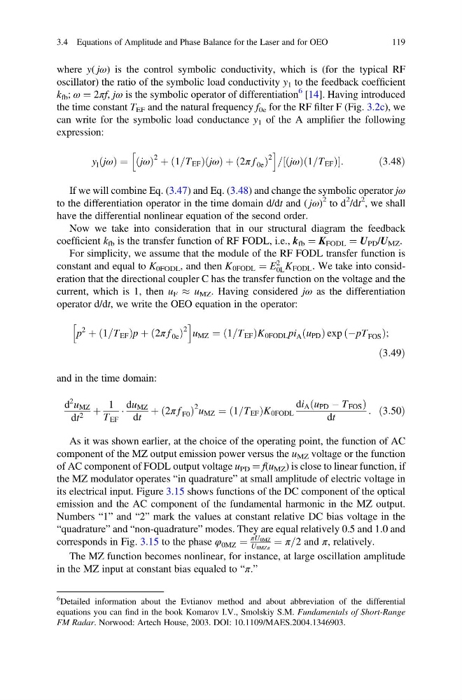
where y( jω) is the control symbolic conductivity, which is (for the typical RF
oscillator) the ratio of the symbolic load conductivity y 1 to the feedback coefficient
k fb ; ω ¼ 2πf, jω is the symbolic operator of differentiation
6 [14]. Having introduced
the time constant T EF and the natural frequency f 0e for the RF filter F (Fig. 3.2c), we
can write for the symbolic load conductance y 1 of the A amplifier the following
expression:
y l jω
ð Þ ¼ jω
ð Þ
2 þ 1=T EF
ð
Þ jω
ð Þ þ 2π f 0e
ð
Þ
2
h
i
= jω
ð Þ 1=T EF
ð
Þ
½
:
ð3:48Þ
If we will combine Eq. (3.47) and Eq. (3.48) and change the symbolic operator jω
to the differentiation operator in the time domain d/dt and ( jω)
2 to d
2 /dt
2 , we shall
have the differential nonlinear equation of the second order.
Now we take into consideration that in our structural diagram the feedback
coefficient k fb is the transfer function of RF FODL, i.e., k fb ¼ K FODL ¼ U PD /U MZ .
For simplicity, we assume that the module of the RF FODL transfer function is
constant and equal to K 0FODL , and then K 0FODL ¼ E
2
0L K FODL . We take into consideration that the directional coupler C has the transfer function on the voltage and the
current, which is 1, then u F % u MZ . Having considered jω as the differentiation
operator d/dt, we write the OEO equation in the operator:
p
2
þ 1=T EF
ð
Þp þ 2π f 0e
ð
Þ
2
h
i
u MZ ¼ 1=T EF
ð
ÞK 0FODL pi A u PD
ð Þexp ÀpT FOS
ð
Þ ;
ð3:49Þ
and in the time domain:
d
2 u MZ
dt 2 þ
1
T EF
Á
du MZ
dt
þ 2π f F0
ð
Þ
2 u MZ ¼ 1=T EF
ð
ÞK 0FODL
di A u PD À T FOS
ð
Þ
dt
: ð3:50Þ
As it was shown earlier, at the choice of the operating point, the function of AC
component of the MZ output emission power versus the u MZ voltage or the function
of AC component of FODL output voltage u PD ¼ f(u MZ ) is close to linear function, if
the MZ modulator operates “in quadrature” at small amplitude of electric voltage in
its electrical input. Figure 3.15 shows functions of the DC component of the optical
emission and the AC component of the fundamental harmonic in the MZ output.
Numbers “1” and “2” mark the values at constant relative DC bias voltage in the
“quadrature” and “non-quadrature” modes. They are equal relatively 0.5 and 1.0 and
corresponds in Fig. 3.15 to the phase φ 0MZ ¼
πU 0MZ
U 0MZπ
¼ π=2 and π, relatively.
The MZ function becomes nonlinear, for instance, at large oscillation amplitude
in the MZ input at constant bias equaled to “π.”
6 Detailed information about the Evtianov method and about abbreviation of the differential
equations you can find in the book Komarov I.V., Smolskiy S.M. Fundamentals of Short-Range
FM Radar. Norwood: Artech House, 2003. DOI: 10.1109/MAES.2004.1346903.
3.4 Equations of Amplitude and Phase Balance for the Laser and for OEO
119
oscillator) the ratio of the symbolic load conductivity y 1 to the feedback coefficient
k fb ; ω ¼ 2πf, jω is the symbolic operator of differentiation
6 [14]. Having introduced
the time constant T EF and the natural frequency f 0e for the RF filter F (Fig. 3.2c), we
can write for the symbolic load conductance y 1 of the A amplifier the following
expression:
y l jω
ð Þ ¼ jω
ð Þ
2 þ 1=T EF
ð
Þ jω
ð Þ þ 2π f 0e
ð
Þ
2
h
i
= jω
ð Þ 1=T EF
ð
Þ
½
:
ð3:48Þ
If we will combine Eq. (3.47) and Eq. (3.48) and change the symbolic operator jω
to the differentiation operator in the time domain d/dt and ( jω)
2 to d
2 /dt
2 , we shall
have the differential nonlinear equation of the second order.
Now we take into consideration that in our structural diagram the feedback
coefficient k fb is the transfer function of RF FODL, i.e., k fb ¼ K FODL ¼ U PD /U MZ .
For simplicity, we assume that the module of the RF FODL transfer function is
constant and equal to K 0FODL , and then K 0FODL ¼ E
2
0L K FODL . We take into consideration that the directional coupler C has the transfer function on the voltage and the
current, which is 1, then u F % u MZ . Having considered jω as the differentiation
operator d/dt, we write the OEO equation in the operator:
p
2
þ 1=T EF
ð
Þp þ 2π f 0e
ð
Þ
2
h
i
u MZ ¼ 1=T EF
ð
ÞK 0FODL pi A u PD
ð Þexp ÀpT FOS
ð
Þ ;
ð3:49Þ
and in the time domain:
d
2 u MZ
dt 2 þ
1
T EF
Á
du MZ
dt
þ 2π f F0
ð
Þ
2 u MZ ¼ 1=T EF
ð
ÞK 0FODL
di A u PD À T FOS
ð
Þ
dt
: ð3:50Þ
As it was shown earlier, at the choice of the operating point, the function of AC
component of the MZ output emission power versus the u MZ voltage or the function
of AC component of FODL output voltage u PD ¼ f(u MZ ) is close to linear function, if
the MZ modulator operates “in quadrature” at small amplitude of electric voltage in
its electrical input. Figure 3.15 shows functions of the DC component of the optical
emission and the AC component of the fundamental harmonic in the MZ output.
Numbers “1” and “2” mark the values at constant relative DC bias voltage in the
“quadrature” and “non-quadrature” modes. They are equal relatively 0.5 and 1.0 and
corresponds in Fig. 3.15 to the phase φ 0MZ ¼
πU 0MZ
U 0MZπ
¼ π=2 and π, relatively.
The MZ function becomes nonlinear, for instance, at large oscillation amplitude
in the MZ input at constant bias equaled to “π.”
6 Detailed information about the Evtianov method and about abbreviation of the differential
equations you can find in the book Komarov I.V., Smolskiy S.M. Fundamentals of Short-Range
FM Radar. Norwood: Artech House, 2003. DOI: 10.1109/MAES.2004.1346903.
3.4 Equations of Amplitude and Phase Balance for the Laser and for OEO
119