

426
10 The Statistical Basis of Bioenergetics
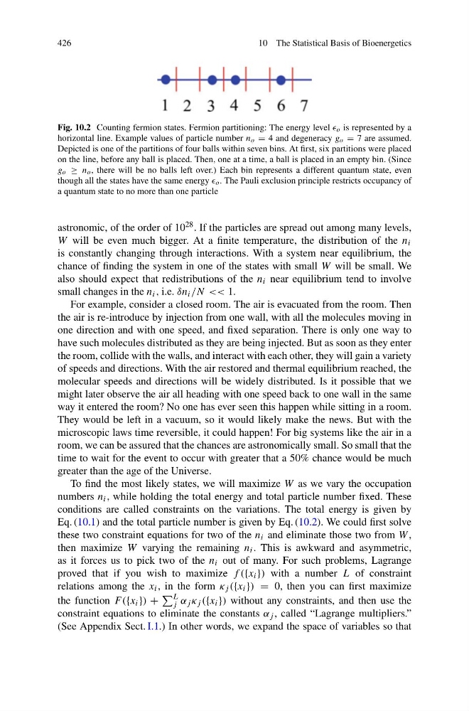
Fig. 10.2 Counting fermion states. Fermion partitioning: The energy level o is represented by a
horizontal line. Example values of particle number n o = 4 and degeneracy g o = 7 are assumed.
Depicted is one of the partitions of four balls within seven bins. At first, six partitions were placed
on the line, before any ball is placed. Then, one at a time, a ball is placed in an empty bin. (Since
g o ≥ n o , there will be no balls left over.) Each bin represents a different quantum state, even
though all the states have the same energy o . The Pauli exclusion principle restricts occupancy of
a quantum state to no more than one particle
astronomic, of the order of 10 28 . If the particles are spread out among many levels,
W will be even much bigger. At a finite temperature, the distribution of the n i
is constantly changing through interactions. With a system near equilibrium, the
chance of finding the system in one of the states with small W will be small. We
also should expect that redistributions of the n i near equilibrium tend to involve
small changes in the n i , i.e. δn i /N << 1.
For example, consider a closed room. The air is evacuated from the room. Then
the air is re-introduce by injection from one wall, with all the molecules moving in
one direction and with one speed, and fixed separation. There is only one way to
have such molecules distributed as they are being injected. But as soon as they enter
the room, collide with the walls, and interact with each other, they will gain a variety
of speeds and directions. With the air restored and thermal equilibrium reached, the
molecular speeds and directions will be widely distributed. Is it possible that we
might later observe the air all heading with one speed back to one wall in the same
way it entered the room? No one has ever seen this happen while sitting in a room.
They would be left in a vacuum, so it would likely make the news. But with the
microscopic laws time reversible, it could happen! For big systems like the air in a
room, we can be assured that the chances are astronomically small. So small that the
time to wait for the event to occur with greater that a 50% chance would be much
greater than the age of the Universe.
To find the most likely states, we will maximize W as we vary the occupation
numbers n i , while holding the total energy and total particle number fixed. These
conditions are called constraints on the variations. The total energy is given by
Eq. (10.1) and the total particle number is given by Eq. (10.2). We could first solve
these two constraint equations for two of the n i and eliminate those two from W ,
then maximize W varying the remaining n i . This is awkward and asymmetric,
as it forces us to pick two of the n i out of many. For such problems, Lagrange
proved that if you wish to maximize f ({x i }) with a number L of constraint
relations among the x i , in the form κ j ({x i }) = 0, then you can first maximize
the function F ({x i }) +
L
j α j κ j ({x i }) without any constraints, and then use the
constraint equations to eliminate the constants α j , called “Lagrange multipliers.”
(See Appendix Sect. I.1.) In other words, we expand the space of variables so that
10 The Statistical Basis of Bioenergetics
Fig. 10.2 Counting fermion states. Fermion partitioning: The energy level o is represented by a
horizontal line. Example values of particle number n o = 4 and degeneracy g o = 7 are assumed.
Depicted is one of the partitions of four balls within seven bins. At first, six partitions were placed
on the line, before any ball is placed. Then, one at a time, a ball is placed in an empty bin. (Since
g o ≥ n o , there will be no balls left over.) Each bin represents a different quantum state, even
though all the states have the same energy o . The Pauli exclusion principle restricts occupancy of
a quantum state to no more than one particle
astronomic, of the order of 10 28 . If the particles are spread out among many levels,
W will be even much bigger. At a finite temperature, the distribution of the n i
is constantly changing through interactions. With a system near equilibrium, the
chance of finding the system in one of the states with small W will be small. We
also should expect that redistributions of the n i near equilibrium tend to involve
small changes in the n i , i.e. δn i /N << 1.
For example, consider a closed room. The air is evacuated from the room. Then
the air is re-introduce by injection from one wall, with all the molecules moving in
one direction and with one speed, and fixed separation. There is only one way to
have such molecules distributed as they are being injected. But as soon as they enter
the room, collide with the walls, and interact with each other, they will gain a variety
of speeds and directions. With the air restored and thermal equilibrium reached, the
molecular speeds and directions will be widely distributed. Is it possible that we
might later observe the air all heading with one speed back to one wall in the same
way it entered the room? No one has ever seen this happen while sitting in a room.
They would be left in a vacuum, so it would likely make the news. But with the
microscopic laws time reversible, it could happen! For big systems like the air in a
room, we can be assured that the chances are astronomically small. So small that the
time to wait for the event to occur with greater that a 50% chance would be much
greater than the age of the Universe.
To find the most likely states, we will maximize W as we vary the occupation
numbers n i , while holding the total energy and total particle number fixed. These
conditions are called constraints on the variations. The total energy is given by
Eq. (10.1) and the total particle number is given by Eq. (10.2). We could first solve
these two constraint equations for two of the n i and eliminate those two from W ,
then maximize W varying the remaining n i . This is awkward and asymmetric,
as it forces us to pick two of the n i out of many. For such problems, Lagrange
proved that if you wish to maximize f ({x i }) with a number L of constraint
relations among the x i , in the form κ j ({x i }) = 0, then you can first maximize
the function F ({x i }) +
L
j α j κ j ({x i }) without any constraints, and then use the
constraint equations to eliminate the constants α j , called “Lagrange multipliers.”
(See Appendix Sect. I.1.) In other words, we expand the space of variables so that