

9.19 Osmosis and Osmotic Pressure
377
With a balancing of chemical potentials for the water (Eq. (9.136)) we find
V c p + RT ln x
w
c = 0 .
(9.140)
Specializing further, we apply x w
c = 1 − x s
c for small concentrations of solute.
This makes the approximation ln (1 − x) = −x reasonable. Also, as water is nearly
incompressible,
V c ≡ ∂V c /∂n c = ∂(M c n c /ρ c )/∂n c = V c /n c .
With the definition of concentration of the solute as C s
c ≡ n s
c /V c = x s
c /(V c /n c ), we
have, finally,
p = RT [C
s
c ] .
(9.141)
[C s
c ] is the molar concentration of the solute. We started with the concentration of
the solute outside taken zero: [C s
b ] = 0. If we had put the cell in a solution of the
same solute, but different concentration than the interior of the cell, then we would
have gotten the more general expression
p = RT
[C
s
c ] − [C
s
b ]
= RT T[C c ] .
(9.142)
We have that the osmotic pressure is proportional to the concentration gradient of
the solute. (This relationship was presented by van’t Hoff in 1884 and so is named
after him.) For non-ideal solutions, wherein interactions between solute particles
come to play, the osmotic pressure may depend non-linearly on the concentration
gradient of the solute.
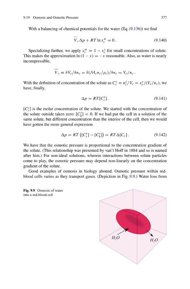
Good examples of osmosis in biology abound. Osmotic pressure within redblood cells varies as they transport gases. (Depiction in Fig. 9.9.) Water loss from
Fig. 9.9 Osmosis of water
into a red-blood cell
377
With a balancing of chemical potentials for the water (Eq. (9.136)) we find
V c p + RT ln x
w
c = 0 .
(9.140)
Specializing further, we apply x w
c = 1 − x s
c for small concentrations of solute.
This makes the approximation ln (1 − x) = −x reasonable. Also, as water is nearly
incompressible,
V c ≡ ∂V c /∂n c = ∂(M c n c /ρ c )/∂n c = V c /n c .
With the definition of concentration of the solute as C s
c ≡ n s
c /V c = x s
c /(V c /n c ), we
have, finally,
p = RT [C
s
c ] .
(9.141)
[C s
c ] is the molar concentration of the solute. We started with the concentration of
the solute outside taken zero: [C s
b ] = 0. If we had put the cell in a solution of the
same solute, but different concentration than the interior of the cell, then we would
have gotten the more general expression
p = RT
[C
s
c ] − [C
s
b ]
= RT T[C c ] .
(9.142)
We have that the osmotic pressure is proportional to the concentration gradient of
the solute. (This relationship was presented by van’t Hoff in 1884 and so is named
after him.) For non-ideal solutions, wherein interactions between solute particles
come to play, the osmotic pressure may depend non-linearly on the concentration
gradient of the solute.
Good examples of osmosis in biology abound. Osmotic pressure within redblood cells varies as they transport gases. (Depiction in Fig. 9.9.) Water loss from
Fig. 9.9 Osmosis of water
into a red-blood cell