

4.2 Open String
59
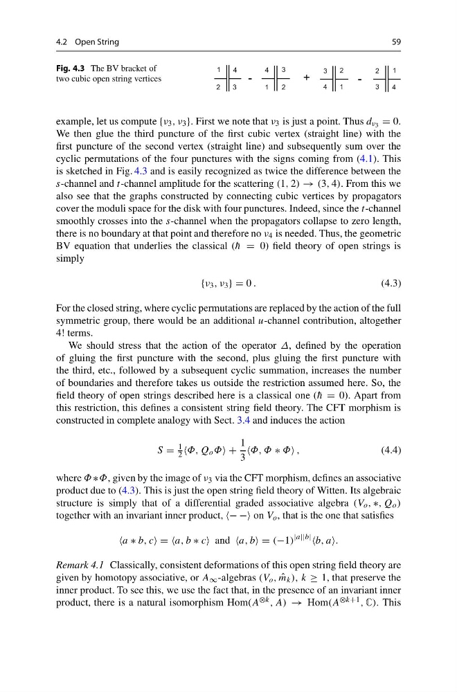
Fig. 4.3 The BV bracket of
two cubic open string vertices
example, let us compute {ν 3 , ν 3 }. First we note that ν 3 is just a point. Thus d ν 3 = 0.
We then glue the third puncture of the first cubic vertex (straight line) with the
first puncture of the second vertex (straight line) and subsequently sum over the
cyclic permutations of the four punctures with the signs coming from (4.1). This
is sketched in Fig. 4.3 and is easily recognized as twice the difference between the
s-channel and t-channel amplitude for the scattering (1, 2) → (3, 4). From this we
also see that the graphs constructed by connecting cubic vertices by propagators
cover the moduli space for the disk with four punctures. Indeed, since the t-channel
smoothly crosses into the s-channel when the propagators collapse to zero length,
there is no boundary at that point and therefore no ν 4 is needed. Thus, the geometric
BV equation that underlies the classical ( ¯
h = 0) field theory of open strings is
simply
{ν 3 , ν 3 } = 0 .
(4.3)
For the closed string, where cyclic permutations are replaced by the action of the full
symmetric group, there would be an additional u-channel contribution, altogether
4! terms.
We should stress that the action of the operator Δ, defined by the operation
of gluing the first puncture with the second, plus gluing the first puncture with
the third, etc., followed by a subsequent cyclic summation, increases the number
of boundaries and therefore takes us outside the restriction assumed here. So, the
field theory of open strings described here is a classical one ( ¯
h = 0). Apart from
this restriction, this defines a consistent string field theory. The CFT morphism is
constructed in complete analogy with Sect. 3.4 and induces the action
S =
1
2 Φ, Q o Φ +
1
3
Φ, Φ ∗ Φ ,
(4.4)
where Φ ∗Φ, given by the image of ν 3 via the CFT morphism, defines an associative
product due to (4.3). This is just the open string field theory of Witten. Its algebraic
structure is simply that of a differential graded associative algebra (V o , ∗, Q o )
together with an invariant inner product, − −− on V o , that is the one that satisfies
∗ b, c = =a, b ∗ c and a, b = (−1)
|a||b|
b, a
Remark 4.1 Classically, consistent deformations of this open string field theory are
given by homotopy associative, or A ∞ -algebras (V o , ˆ
m k ), k ≥ 1, that preserve the
inner product. To see this, we use the fact that, in the presence of an invariant inner
product, there is a natural isomorphism Hom(A ⊗k , A) → Hom(A ⊗k+1 , C). This
59
Fig. 4.3 The BV bracket of
two cubic open string vertices
example, let us compute {ν 3 , ν 3 }. First we note that ν 3 is just a point. Thus d ν 3 = 0.
We then glue the third puncture of the first cubic vertex (straight line) with the
first puncture of the second vertex (straight line) and subsequently sum over the
cyclic permutations of the four punctures with the signs coming from (4.1). This
is sketched in Fig. 4.3 and is easily recognized as twice the difference between the
s-channel and t-channel amplitude for the scattering (1, 2) → (3, 4). From this we
also see that the graphs constructed by connecting cubic vertices by propagators
cover the moduli space for the disk with four punctures. Indeed, since the t-channel
smoothly crosses into the s-channel when the propagators collapse to zero length,
there is no boundary at that point and therefore no ν 4 is needed. Thus, the geometric
BV equation that underlies the classical ( ¯
h = 0) field theory of open strings is
simply
{ν 3 , ν 3 } = 0 .
(4.3)
For the closed string, where cyclic permutations are replaced by the action of the full
symmetric group, there would be an additional u-channel contribution, altogether
4! terms.
We should stress that the action of the operator Δ, defined by the operation
of gluing the first puncture with the second, plus gluing the first puncture with
the third, etc., followed by a subsequent cyclic summation, increases the number
of boundaries and therefore takes us outside the restriction assumed here. So, the
field theory of open strings described here is a classical one ( ¯
h = 0). Apart from
this restriction, this defines a consistent string field theory. The CFT morphism is
constructed in complete analogy with Sect. 3.4 and induces the action
S =
1
2 Φ, Q o Φ +
1
3
Φ, Φ ∗ Φ ,
(4.4)
where Φ ∗Φ, given by the image of ν 3 via the CFT morphism, defines an associative
product due to (4.3). This is just the open string field theory of Witten. Its algebraic
structure is simply that of a differential graded associative algebra (V o , ∗, Q o )
together with an invariant inner product, − −− on V o , that is the one that satisfies
∗ b, c = =a, b ∗ c and a, b = (−1)
|a||b|
b, a
Remark 4.1 Classically, consistent deformations of this open string field theory are
given by homotopy associative, or A ∞ -algebras (V o , ˆ
m k ), k ≥ 1, that preserve the
inner product. To see this, we use the fact that, in the presence of an invariant inner
product, there is a natural isomorphism Hom(A ⊗k , A) → Hom(A ⊗k+1 , C). This