

180
7 Feynman Transform of a Modular Operad
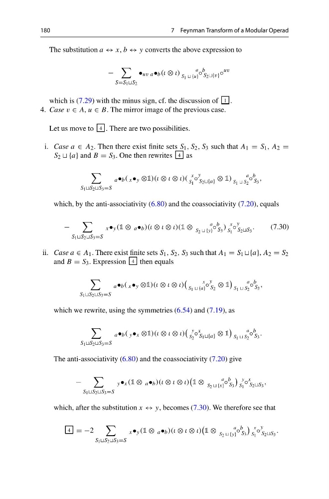
The substitution a ↔ x, b ↔ y converts the above expression to
−
S=S 1 2
• uv a • b (ι ⊗ ι)
a
S 1 {u}
◦
b
S 2 ◦
uv
which is (7.29) with the minus sign, cf. the discussion of 1 .
4. Case v ∈ A, u ∈ B. The mirror image of the previous case.
Let us move to 4 . There are two possibilities.
i. Case a ∈ A 2 . Then there exist finite sets S 1 , S 2 , S 3 such that A 1 = S 1 , A 2 =
S 2 {a} and B = S 3 . One then rewrites 4 as
S 1 2 3 =S
a • b ( x • y ⊗1)(ι ⊗ ι ⊗ ι)(
x
S 1
◦
y
S 2 ⊗ 1)
a
S 1 S 2
◦
b
S 3
,
which, by the anti-associativity (6.80) and the coassociativity (7.20), equals
−
S 1 2 3 =S
x • y (1 ⊗ a • b )(ι ⊗ ι ⊗ ι)(1 ⊗
a
S 2 {y}
◦
b
S 3
)
x
S 1
◦
y
S 2 3
.
(7.30)
ii. Case a ∈ A 1 . There exist finite sets S 1 , S 2 , S 3 such that A 1 = S 1 A 2 = S 2
and B = S 3 . Expression 4 then equals
S 1 2 3 =S
a • b ( x • y ⊗1)(ι ⊗ ι ⊗ ι)
x
S 1 {a}
◦
y
S 2
⊗ 1
a
S 1 S 2
◦
b
S 3
,
which we rewrite, using the symmetries (6.54) and (7.19), as
S 1 2 3 =S
a • b ( y • x ⊗1)(ι ⊗ ι ⊗ ι)
y
S 2
◦
x
S 1 ⊗ 1
a
S 1 S 2
◦
b
S 3
.
The anti-associativity (6.80) and the coassociativity (7.20) give
−
S 1 2 3 =S
y • x (1 ⊗ a • b )(ι ⊗ ι ⊗ ι)
1 ⊗
a
S 2 {x}
◦
b
S 3
y
S 1
◦
x
S 2 3
,
which, after the substitution x ↔ y, becomes (7.30). We therefore see that
4 = −2
S 1 2 3 =S
x • y (1 ⊗ a • b )(ι ⊗ ι ⊗ ι)
1 ⊗
a
S 2 {y}
◦
b
S 3
x
S 1
◦
y
S 2 3
.
7 Feynman Transform of a Modular Operad
The substitution a ↔ x, b ↔ y converts the above expression to
−
S=S 1 2
• uv a • b (ι ⊗ ι)
a
S 1 {u}
◦
b
S 2 ◦
uv
which is (7.29) with the minus sign, cf. the discussion of 1 .
4. Case v ∈ A, u ∈ B. The mirror image of the previous case.
Let us move to 4 . There are two possibilities.
i. Case a ∈ A 2 . Then there exist finite sets S 1 , S 2 , S 3 such that A 1 = S 1 , A 2 =
S 2 {a} and B = S 3 . One then rewrites 4 as
S 1 2 3 =S
a • b ( x • y ⊗1)(ι ⊗ ι ⊗ ι)(
x
S 1
◦
y
S 2 ⊗ 1)
a
S 1 S 2
◦
b
S 3
,
which, by the anti-associativity (6.80) and the coassociativity (7.20), equals
−
S 1 2 3 =S
x • y (1 ⊗ a • b )(ι ⊗ ι ⊗ ι)(1 ⊗
a
S 2 {y}
◦
b
S 3
)
x
S 1
◦
y
S 2 3
.
(7.30)
ii. Case a ∈ A 1 . There exist finite sets S 1 , S 2 , S 3 such that A 1 = S 1 A 2 = S 2
and B = S 3 . Expression 4 then equals
S 1 2 3 =S
a • b ( x • y ⊗1)(ι ⊗ ι ⊗ ι)
x
S 1 {a}
◦
y
S 2
⊗ 1
a
S 1 S 2
◦
b
S 3
,
which we rewrite, using the symmetries (6.54) and (7.19), as
S 1 2 3 =S
a • b ( y • x ⊗1)(ι ⊗ ι ⊗ ι)
y
S 2
◦
x
S 1 ⊗ 1
a
S 1 S 2
◦
b
S 3
.
The anti-associativity (6.80) and the coassociativity (7.20) give
−
S 1 2 3 =S
y • x (1 ⊗ a • b )(ι ⊗ ι ⊗ ι)
1 ⊗
a
S 2 {x}
◦
b
S 3
y
S 1
◦
x
S 2 3
,
which, after the substitution x ↔ y, becomes (7.30). We therefore see that
4 = −2
S 1 2 3 =S
x • y (1 ⊗ a • b )(ι ⊗ ι ⊗ ι)
1 ⊗
a
S 2 {y}
◦
b
S 3
x
S 1
◦
y
S 2 3
.