

6.1 Cyclic Operads
123
be the extension of the identity map 1 : P → P of cyclic modules. For a tree T
with Leg(T ) = S we define the contraction along T as the composition
c T : P(T )
i T
−→ F(P)(S)
Π
−→ P(S)
(6.37)
of Π with the canonical map (6.35).
Let us indicate an explicit construction of c T by induction on the number of the
edges of T . If T is a corolla S , P( S ) = P(S) and we put c T =: 1 S . Each tree T
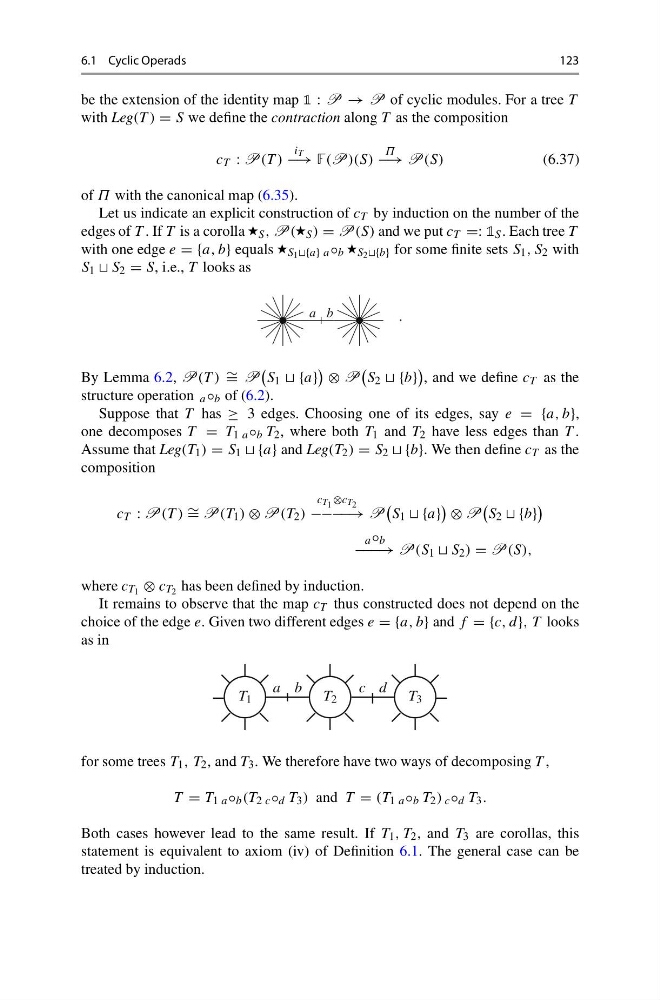
with one edge e = {a, b} equals S 1 a ◦ b S 2 for some finite sets S 1 , S 2 with
S 1 S 2 = S, i.e., T looks as
a b
.
By Lemma 6.2, P(T ) ∼ = P
S 1 {a}
⊗ P
S 2 {b}
, and we define c T as the
structure operation a ◦ b of (6.2).
Suppose that T has ≥ 3 edges. Choosing one of its edges, say e = {a, b},
one decomposes T = T 1 a ◦ b T 2 , where both T 1 and T 2 have less edges than T .
Assume that Leg(T 1 ) = S 1 {a} and Leg(T 2 ) = S 2 {b}. We then define c T as the
composition
c T : P(T ) ∼ = P(T 1 ) ⊗ P(T 2 )
c T 1 ⊗c T 2
−−−−→ P
S 1 {a}
⊗ P
S 2 {b}
a ◦ b
−−−→ P(S 1 S 2 ) = P(S),
where c T 1 ⊗ c T 2 has been defined by induction.
It remains to observe that the map c T thus constructed does not depend on the
choice of the edge e. Given two different edges e = {a, b} and f = {c, d}, T looks
as in
T 1
T 2
a b
T 3
c d
for some trees T 1 , T 2 , and T 3 . We therefore have two ways of decomposing T ,
T = T 1 a ◦ b (T 2 c ◦ d T 3 ) and T = (T 1 a ◦ b T 2 ) c ◦ d T 3 .
Both cases however lead to the same result. If T 1 , T 2 , and T 3 are corollas, this
statement is equivalent to axiom (iv) of Definition 6.1. The general case can be
treated by induction.
123
be the extension of the identity map 1 : P → P of cyclic modules. For a tree T
with Leg(T ) = S we define the contraction along T as the composition
c T : P(T )
i T
−→ F(P)(S)
Π
−→ P(S)
(6.37)
of Π with the canonical map (6.35).
Let us indicate an explicit construction of c T by induction on the number of the
edges of T . If T is a corolla S , P( S ) = P(S) and we put c T =: 1 S . Each tree T
with one edge e = {a, b} equals S 1 a ◦ b S 2 for some finite sets S 1 , S 2 with
S 1 S 2 = S, i.e., T looks as
a b
.
By Lemma 6.2, P(T ) ∼ = P
S 1 {a}
⊗ P
S 2 {b}
, and we define c T as the
structure operation a ◦ b of (6.2).
Suppose that T has ≥ 3 edges. Choosing one of its edges, say e = {a, b},
one decomposes T = T 1 a ◦ b T 2 , where both T 1 and T 2 have less edges than T .
Assume that Leg(T 1 ) = S 1 {a} and Leg(T 2 ) = S 2 {b}. We then define c T as the
composition
c T : P(T ) ∼ = P(T 1 ) ⊗ P(T 2 )
c T 1 ⊗c T 2
−−−−→ P
S 1 {a}
⊗ P
S 2 {b}
a ◦ b
−−−→ P(S 1 S 2 ) = P(S),
where c T 1 ⊗ c T 2 has been defined by induction.
It remains to observe that the map c T thus constructed does not depend on the
choice of the edge e. Given two different edges e = {a, b} and f = {c, d}, T looks
as in
T 1
T 2
a b
T 3
c d
for some trees T 1 , T 2 , and T 3 . We therefore have two ways of decomposing T ,
T = T 1 a ◦ b (T 2 c ◦ d T 3 ) and T = (T 1 a ◦ b T 2 ) c ◦ d T 3 .
Both cases however lead to the same result. If T 1 , T 2 , and T 3 are corollas, this
statement is equivalent to axiom (iv) of Definition 6.1. The general case can be
treated by induction.