

334
17 Blouin Zones, Effective Mass, Muffin-tin Potential…
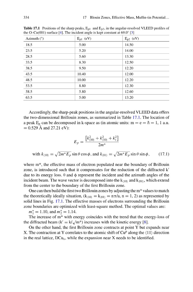
Table 17.1 Positions of the sharp peaks, E p1 and E p2 , in the angular-resolved VLEED profiles of
the O–Cu(001) surface [4]. The incident angle is kept constant at 69.0° [3]
Azimuth (°)
E p1 (eV)
E p2 (eV)
18.5
5.00
14.50
23.5
5.20
14.00
28.5
5.60
13.30
33.5
8.30
12.50
38.5
9.50
12.20
43.5
10.40
12.00
48.5
10.00
12.20
53.5
8.80
12.30
58.5
5.80
12.60
63.5
5.00
13.20
Accordingly, the sharp-peak positions in the angular-resolved VLEED data offers
the two-dimensional Brillouin zones, as summarized in Table 17.1. The location of
a peak E p can be decomposed in k-space as (in atomic units: m = e = = 1, 1 a.u.
= 0.529 Å and 27.21 eV):
E p =
k
2
10 + k
2
10 + k
2
z
2m ∗
with k 10 =
2m ∗ E p sin θ cos φ, and k 01 =
2m ∗ E p sin θ sin φ,
(17.1)
where m*, the effective mass of electron populated near the boundary of Brillouin
zone, is introduced such that it compensates for the reduction of the diffracted k
due to its energy loss. θ and φ represent the incident and the azimuth angles of the
incident beam. The wave vector is decomposed into the k 10 and k 01 , which extend
from the center to the boundary of the first Brillouin zone.
One can then build the first two Brillouin zones by adjusting the m* values to match
the theoretically ideally situation, (k 10 = k 01 = nπ/a, n = 1, 2) as represented by
solid lines in Fig. 17.1. The effective masses of electrons surrounding the Brillouin
zone boundaries are optimized with least-square method. The optimal values are:
m
∗
1 = 1.10, and m
∗
2 = 1.14.
The increase of m* with energy coincides with the trend that the energy-loss of
the diffracted beam (k
= k/
√
m*) increases with the kinetic energy [8].
On the other hand, the first Brillouin zone contracts at point Y but expands near
X. The contraction at Y correlates to the atomic shift of Cu
p along the 11 direction
in the real lattice, DCu x , while the expansion near X needs to be identified.
17 Blouin Zones, Effective Mass, Muffin-tin Potential…
Table 17.1 Positions of the sharp peaks, E p1 and E p2 , in the angular-resolved VLEED profiles of
the O–Cu(001) surface [4]. The incident angle is kept constant at 69.0° [3]
Azimuth (°)
E p1 (eV)
E p2 (eV)
18.5
5.00
14.50
23.5
5.20
14.00
28.5
5.60
13.30
33.5
8.30
12.50
38.5
9.50
12.20
43.5
10.40
12.00
48.5
10.00
12.20
53.5
8.80
12.30
58.5
5.80
12.60
63.5
5.00
13.20
Accordingly, the sharp-peak positions in the angular-resolved VLEED data offers
the two-dimensional Brillouin zones, as summarized in Table 17.1. The location of
a peak E p can be decomposed in k-space as (in atomic units: m = e = = 1, 1 a.u.
= 0.529 Å and 27.21 eV):
E p =
k
2
10 + k
2
10 + k
2
z
2m ∗
with k 10 =
2m ∗ E p sin θ cos φ, and k 01 =
2m ∗ E p sin θ sin φ,
(17.1)
where m*, the effective mass of electron populated near the boundary of Brillouin
zone, is introduced such that it compensates for the reduction of the diffracted k
due to its energy loss. θ and φ represent the incident and the azimuth angles of the
incident beam. The wave vector is decomposed into the k 10 and k 01 , which extend
from the center to the boundary of the first Brillouin zone.
One can then build the first two Brillouin zones by adjusting the m* values to match
the theoretically ideally situation, (k 10 = k 01 = nπ/a, n = 1, 2) as represented by
solid lines in Fig. 17.1. The effective masses of electrons surrounding the Brillouin
zone boundaries are optimized with least-square method. The optimal values are:
m
∗
1 = 1.10, and m
∗
2 = 1.14.
The increase of m* with energy coincides with the trend that the energy-loss of
the diffracted beam (k
= k/
√
m*) increases with the kinetic energy [8].
On the other hand, the first Brillouin zone contracts at point Y but expands near
X. The contraction at Y correlates to the atomic shift of Cu
p along the 11 direction
in the real lattice, DCu x , while the expansion near X needs to be identified.