

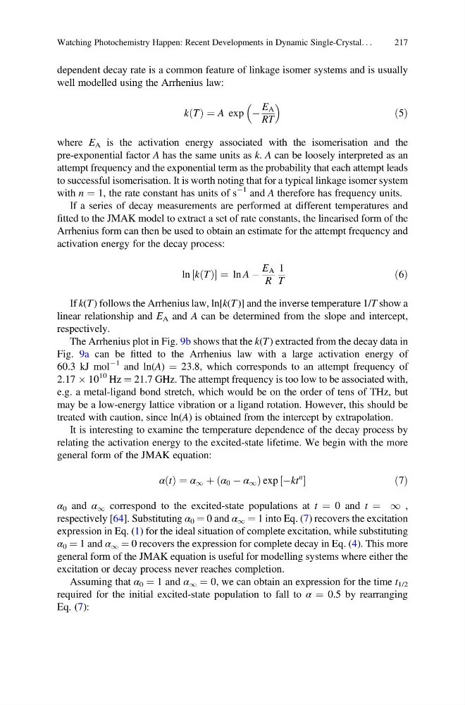
dependent decay rate is a common feature of linkage isomer systems and is usually
well modelled using the Arrhenius law:
k T
ð Þ ¼ A exp À
E A
RT
ð5Þ
where E A is the activation energy associated with the isomerisation and the
pre-exponential factor A has the same units as k. A can be loosely interpreted as an
attempt frequency and the exponential term as the probability that each attempt leads
to successful isomerisation. It is worth noting that for a typical linkage isomer system
with n ¼ 1, the rate constant has units of s
À1 and A therefore has frequency units.
If a series of decay measurements are performed at different temperatures and
fitted to the JMAK model to extract a set of rate constants, the linearised form of the
Arrhenius form can then be used to obtain an estimate for the attempt frequency and
activation energy for the decay process:
ln k T
ð Þ
½
¼ ln A À
E A
R
1
T
ð6Þ
If k(T ) follows the Arrhenius law, ln[k(T )] and the inverse temperature 1/T show a
linear relationship and E A and A can be determined from the slope and intercept,
respectively.
The Arrhenius plot in Fig. 9b shows that the k(T ) extracted from the decay data in
Fig. 9a can be fitted to the Arrhenius law with a large activation energy of
60.3 kJ mol
À1 and ln(A) ¼ 23.8, which corresponds to an attempt frequency of
2.17 Â 10
10 Hz ¼ 21.7 GHz. The attempt frequency is too low to be associated with,
e.g. a metal-ligand bond stretch, which would be on the order of tens of THz, but
may be a low-energy lattice vibration or a ligand rotation. However, this should be
treated with caution, since ln(A) is obtained from the intercept by extrapolation.
It is interesting to examine the temperature dependence of the decay process by
relating the activation energy to the excited-state lifetime. We begin with the more
general form of the JMAK equation:
α t
ð Þ ¼ α 1 þ α 0 À α 1
ð
Þexp Àkt
n
½
ð7Þ
α 0 and α 1 correspond to the excited-state populations at t ¼ 0 and t ¼ 1 ,
respectively [64]. Substituting α 0 ¼ 0 and α 1 ¼ 1 into Eq. (7) recovers the excitation
expression in Eq. (1) for the ideal situation of complete excitation, while substituting
α 0 ¼ 1 and α 1 ¼ 0 recovers the expression for complete decay in Eq. (4). This more
general form of the JMAK equation is useful for modelling systems where either the
excitation or decay process never reaches completion.
Assuming that α 0 ¼ 1 and α 1 ¼ 0, we can obtain an expression for the time t 1/2
required for the initial excited-state population to fall to α ¼ 0.5 by rearranging
Eq. (7):
Watching Photochemistry Happen: Recent Developments in Dynamic Single-Crystal. . .
217
well modelled using the Arrhenius law:
k T
ð Þ ¼ A exp À
E A
RT
ð5Þ
where E A is the activation energy associated with the isomerisation and the
pre-exponential factor A has the same units as k. A can be loosely interpreted as an
attempt frequency and the exponential term as the probability that each attempt leads
to successful isomerisation. It is worth noting that for a typical linkage isomer system
with n ¼ 1, the rate constant has units of s
À1 and A therefore has frequency units.
If a series of decay measurements are performed at different temperatures and
fitted to the JMAK model to extract a set of rate constants, the linearised form of the
Arrhenius form can then be used to obtain an estimate for the attempt frequency and
activation energy for the decay process:
ln k T
ð Þ
½
¼ ln A À
E A
R
1
T
ð6Þ
If k(T ) follows the Arrhenius law, ln[k(T )] and the inverse temperature 1/T show a
linear relationship and E A and A can be determined from the slope and intercept,
respectively.
The Arrhenius plot in Fig. 9b shows that the k(T ) extracted from the decay data in
Fig. 9a can be fitted to the Arrhenius law with a large activation energy of
60.3 kJ mol
À1 and ln(A) ¼ 23.8, which corresponds to an attempt frequency of
2.17 Â 10
10 Hz ¼ 21.7 GHz. The attempt frequency is too low to be associated with,
e.g. a metal-ligand bond stretch, which would be on the order of tens of THz, but
may be a low-energy lattice vibration or a ligand rotation. However, this should be
treated with caution, since ln(A) is obtained from the intercept by extrapolation.
It is interesting to examine the temperature dependence of the decay process by
relating the activation energy to the excited-state lifetime. We begin with the more
general form of the JMAK equation:
α t
ð Þ ¼ α 1 þ α 0 À α 1
ð
Þexp Àkt
n
½
ð7Þ
α 0 and α 1 correspond to the excited-state populations at t ¼ 0 and t ¼ 1 ,
respectively [64]. Substituting α 0 ¼ 0 and α 1 ¼ 1 into Eq. (7) recovers the excitation
expression in Eq. (1) for the ideal situation of complete excitation, while substituting
α 0 ¼ 1 and α 1 ¼ 0 recovers the expression for complete decay in Eq. (4). This more
general form of the JMAK equation is useful for modelling systems where either the
excitation or decay process never reaches completion.
Assuming that α 0 ¼ 1 and α 1 ¼ 0, we can obtain an expression for the time t 1/2
required for the initial excited-state population to fall to α ¼ 0.5 by rearranging
Eq. (7):
Watching Photochemistry Happen: Recent Developments in Dynamic Single-Crystal. . .
217