

7 Vlse Criterion Optimization and Compromise Solution …
45
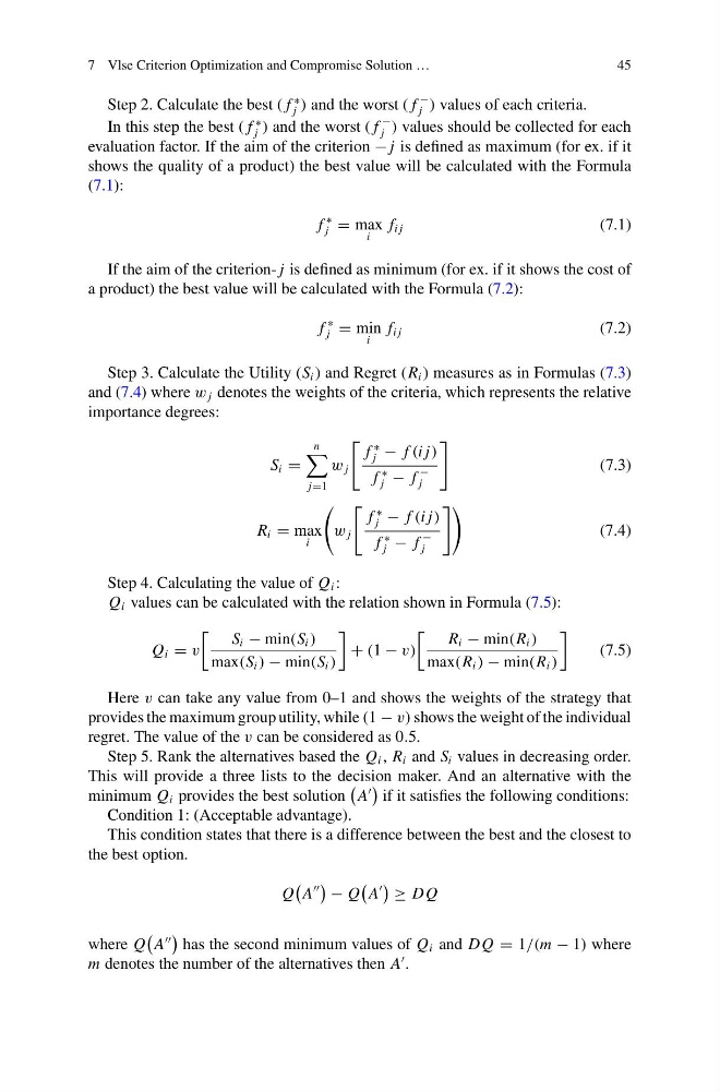
Step 2. Calculate the best ( f
∗
j ) and the worst ( f
−
j ) values of each criteria.
In this step the best ( f
∗
j ) and the worst ( f
−
j ) values should be collected for each
evaluation factor. If the aim of the criterion − j is defined as maximum (for ex. if it
shows the quality of a product) the best value will be calculated with the Formula
(7.1):
f
∗
j = max
i
f i j
(7.1)
If the aim of the criterion- j is defined as minimum (for ex. if it shows the cost of
a product) the best value will be calculated with the Formula (7.2):
f
∗
j = min
i
f i j
(7.2)
Step 3. Calculate the Utility (S i ) and Regret (R i ) measures as in Formulas (7.3)
and (7.4) where w j denotes the weights of the criteria, which represents the relative
importance degrees:
S i =
n
j=1
w j
f
∗
j − f (i j)
f
∗
j − f
−
j
(7.3)
R i = max
i
w j
f
∗
j − f (i j)
f
∗
j − f
−
j
(7.4)
Step 4. Calculating the value of Q i :
Q i values can be calculated with the relation shown in Formula (7.5):
Q i = v
S i − min(S i )
max(S i ) − min(S i )
+ (1 − v)
R i − min(R i )
max(R i ) − min(R i )
(7.5)
Here v can take any value from 0–1 and shows the weights of the strategy that
provides the maximum group utility, while (1 − v) shows the weight of the individual
regret. The value of the v can be considered as 0.5.
Step 5. Rank the alternatives based the Q i , R i and S i values in decreasing order.
This will provide a three lists to the decision maker. And an alternative with the
minimum Q i provides the best solution
A
if it satisfies the following conditions:
Condition 1: (Acceptable advantage).
This condition states that there is a difference between the best and the closest to
the best option.
Q
A
− Q
A
≥ D Q
where Q
A
has the second minimum values of Q i and D Q = 1/(m − 1) where
m denotes the number of the alternatives then A
.
45
Step 2. Calculate the best ( f
∗
j ) and the worst ( f
−
j ) values of each criteria.
In this step the best ( f
∗
j ) and the worst ( f
−
j ) values should be collected for each
evaluation factor. If the aim of the criterion − j is defined as maximum (for ex. if it
shows the quality of a product) the best value will be calculated with the Formula
(7.1):
f
∗
j = max
i
f i j
(7.1)
If the aim of the criterion- j is defined as minimum (for ex. if it shows the cost of
a product) the best value will be calculated with the Formula (7.2):
f
∗
j = min
i
f i j
(7.2)
Step 3. Calculate the Utility (S i ) and Regret (R i ) measures as in Formulas (7.3)
and (7.4) where w j denotes the weights of the criteria, which represents the relative
importance degrees:
S i =
n
j=1
w j
f
∗
j − f (i j)
f
∗
j − f
−
j
(7.3)
R i = max
i
w j
f
∗
j − f (i j)
f
∗
j − f
−
j
(7.4)
Step 4. Calculating the value of Q i :
Q i values can be calculated with the relation shown in Formula (7.5):
Q i = v
S i − min(S i )
max(S i ) − min(S i )
+ (1 − v)
R i − min(R i )
max(R i ) − min(R i )
(7.5)
Here v can take any value from 0–1 and shows the weights of the strategy that
provides the maximum group utility, while (1 − v) shows the weight of the individual
regret. The value of the v can be considered as 0.5.
Step 5. Rank the alternatives based the Q i , R i and S i values in decreasing order.
This will provide a three lists to the decision maker. And an alternative with the
minimum Q i provides the best solution
A
if it satisfies the following conditions:
Condition 1: (Acceptable advantage).
This condition states that there is a difference between the best and the closest to
the best option.
Q
A
− Q
A
≥ D Q
where Q
A
has the second minimum values of Q i and D Q = 1/(m − 1) where
m denotes the number of the alternatives then A
.