

K ¼ 8
a 0
ε p
, I n ¼
4
ε p
p t n
ð Þ, ϕ n ¼ t n
ð9:7:5Þ
It is well-known that the simple Eq. (9.7.4) has the threshold value of K over
which the solution becomes chaos. The chaos solution is given [27] for
K > 1
ð9:7:6Þ
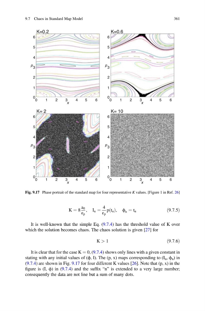
It is clear that for the case K ¼ 0, (9.7.4) shows only lines with a given constant in
stating with any initial values of (ϕ, I). The (p, x) maps corresponding to (I n , ϕ n ) in
(9.7.4) are shown in Fig. 9.17 for four different K values [26]. Note that (p, x) in the
figure is (I, ϕ) in (9.7.4) and the suffix “n” is extended to a very large number;
consequently the data are not line but a sum of many dots.
6
K=0.2
5
4
3
p
x
1
0
0
1
2
3
4
5
6
6
K=0.6
5
4
3
p
x
1
0
0
1
2
3
4
5
6
2
6
K= 2
5
4
3
p
x
1
0
0
1
2
3
4
5
6
2
6
K= 10
5
4
3
p
x
1
0
0
1
2
3
4
5
6
2
2
Fig. 9.17 Phase portrait of the standard map for four representative K values. [Figure 1 in Ref. 26]
9.7 Chaos in Standard Map Model
361
a 0
ε p
, I n ¼
4
ε p
p t n
ð Þ, ϕ n ¼ t n
ð9:7:5Þ
It is well-known that the simple Eq. (9.7.4) has the threshold value of K over
which the solution becomes chaos. The chaos solution is given [27] for
K > 1
ð9:7:6Þ
It is clear that for the case K ¼ 0, (9.7.4) shows only lines with a given constant in
stating with any initial values of (ϕ, I). The (p, x) maps corresponding to (I n , ϕ n ) in
(9.7.4) are shown in Fig. 9.17 for four different K values [26]. Note that (p, x) in the
figure is (I, ϕ) in (9.7.4) and the suffix “n” is extended to a very large number;
consequently the data are not line but a sum of many dots.
6
K=0.2
5
4
3
p
x
1
0
0
1
2
3
4
5
6
6
K=0.6
5
4
3
p
x
1
0
0
1
2
3
4
5
6
2
6
K= 2
5
4
3
p
x
1
0
0
1
2
3
4
5
6
2
6
K= 10
5
4
3
p
x
1
0
0
1
2
3
4
5
6
2
2
Fig. 9.17 Phase portrait of the standard map for four representative K values. [Figure 1 in Ref. 26]
9.7 Chaos in Standard Map Model
361