

T h / t
C C ¼ 1=2 ~ 1
À
Á
ð9:4:19Þ
The time dependence of the computational results shown in [5] can be well
explained by the physical model based on FFPE. It is also important to note that
the model simulation with many small kicks in [1] concluded that the effective
temperatures scale roughly as (9.4.17) with time and laser intensity.
Finally, compare the theoretical result with experimental data [17], where Levy’s
jumps are expected in the interaction region, because the pulse lengths are relatively
long, and large amplitude of noise fields are inferred to be generated in the plasma
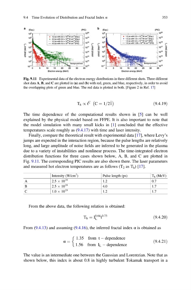
due to a variety of instabilities and nonlinear process. The time-integrated electron
distribution functions for three cases shown below, A, B, and C are plotted in
Fig. 9.11. The corresponding PIC results are also shown there. The laser parameters
and measured hot electron temperatures are as follows (T 2 as T h ) [17].
Intensity (W/cm
2
)
Pulse length (ps)
T h (MeV)
A
2.5 Â 10
18
1.2
0.7
B
2.5 Â 10
18
4.0
1.7
C
1.0 Â 10
19
1.2
1.7
From the above data, the following relation is obtained:
T h ¼ I
0:64
L t
0:73
ð9:4:20Þ
From (9.4.13) and assuming (9.4.16), the inferred fractal index α is obtained as
α ¼
1:35 from t À dependence
1:56 from I L À dependence
&
ð9:4:21Þ
The value is an intermediate one between the Gaussian and Lorentzian. Note that as
shown below, this index is about 0.8 in highly turbulent Tokamak transport in a
Fig. 9.11 Experimental data of the electron energy distributions in three different shots. Three different
shot data A, B, and C are plotted in (a) and (b) with red, green, and blue, respectively, in order to avoid
the overlapping plots of green and blue. The red data is plotted in both. [Figure 2 in Ref. 17]
9.4 Time Evolution of Distribution and Fractal Index α
353
C C ¼ 1=2 ~ 1
À
Á
ð9:4:19Þ
The time dependence of the computational results shown in [5] can be well
explained by the physical model based on FFPE. It is also important to note that
the model simulation with many small kicks in [1] concluded that the effective
temperatures scale roughly as (9.4.17) with time and laser intensity.
Finally, compare the theoretical result with experimental data [17], where Levy’s
jumps are expected in the interaction region, because the pulse lengths are relatively
long, and large amplitude of noise fields are inferred to be generated in the plasma
due to a variety of instabilities and nonlinear process. The time-integrated electron
distribution functions for three cases shown below, A, B, and C are plotted in
Fig. 9.11. The corresponding PIC results are also shown there. The laser parameters
and measured hot electron temperatures are as follows (T 2 as T h ) [17].
Intensity (W/cm
2
)
Pulse length (ps)
T h (MeV)
A
2.5 Â 10
18
1.2
0.7
B
2.5 Â 10
18
4.0
1.7
C
1.0 Â 10
19
1.2
1.7
From the above data, the following relation is obtained:
T h ¼ I
0:64
L t
0:73
ð9:4:20Þ
From (9.4.13) and assuming (9.4.16), the inferred fractal index α is obtained as
α ¼
1:35 from t À dependence
1:56 from I L À dependence
&
ð9:4:21Þ
The value is an intermediate one between the Gaussian and Lorentzian. Note that as
shown below, this index is about 0.8 in highly turbulent Tokamak transport in a
Fig. 9.11 Experimental data of the electron energy distributions in three different shots. Three different
shot data A, B, and C are plotted in (a) and (b) with red, green, and blue, respectively, in order to avoid
the overlapping plots of green and blue. The red data is plotted in both. [Figure 2 in Ref. 17]
9.4 Time Evolution of Distribution and Fractal Index α
353