

condition is modeled in 2D code. In addition, for well computing the nonlinear laser
propagation in pre-formed plasma, laser field is calculated with the vacuum
boundary, 100 μm distant place from the critical surface. A snapshot of laser energy
flux (P laser ; pointing flux), electron density (contour lines), and electron energy flux
(F e ) is shown in Fig. 7.19 for the time of laser power peak. It is seen that the laser
beam are subject to the filamentation instability before arriving at the critical surface.
The brightest filament generates hot electrons into the solid density with wide angle.
The red dotted line is the initial density contours, and the critical surface is found to
have moved about 5 μm, consistent with the distance evaluated from the average
value of the Doppler shift, velocity, in Fig. 7.18. At the time of the laser peak, a sharp
density jump is seen at the critical surface of the brightest filament.
It is pointed out in Ref. [14] that the following simple theoretical model for
energy and momentum balance between laser and plasma well explains the 2D PIC
result. Forget about 2ω component of JxB, and require that the boundary pressure at
the critical surface should satisfy a quasi-static condition:
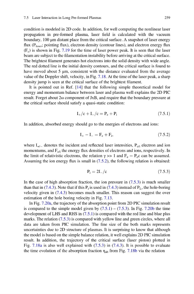
I þ =c þ I À =c ¼ P e þ P i
ð7:5:1Þ
In addition, absorbed energy should go to the energies of electrons and ions:
I þ À I À ¼ F e þ F i ,
ð7:5:2Þ
where I +/À denotes the incident and reflected laser intensities, P e/i electron and ion
momentums, and F e/i the energy flux densities of electrons and ions, respectively. In
the limit of relativistic electrons, the relation γ >> 1 and F e ¼ P e c can be assumed.
Assuming the ion energy flux is small in (7.5.2), the following relation is obtained:
P i ¼ 2I À =c
ð7:5:3Þ
In the case of high absorption fraction, the ion pressure in (7.5.3) is much smaller
than that in (7.4.3). Note that if this P i is used in (7.4.3) instead of P L , the hole-boring
velocity given in (7.4.3) becomes much smaller. This reason can suggest the over
estimation of the hole boring velocity in Fig. 7.13.
In Fig. 7.20a, the trajectory of the absorption point from 2D PIC simulation result
is compared to the simple model given by (7.5.1) – (7.5.3). In Fig. 7.20b the time
development of LHS and RHS in (7.5.1) is compared with the red line and blue plus
marks. The relation (7.5.3) is compared with yellow line and green circles, where all
data are taken from PIC simulation. The fine size of the both marks represents
uncertainties due to 2D structure of plasmas. It is surprising to know that although
the model is based on the simple balance relation, it well explains 2D PIC simulation
result. In addition, the trajectory of the critical surface (laser piston) plotted in
Fig. 7.18a is also well explained with (7.5.3) in (7.4.3). It is possible to evaluate
the time evolution of the absorption fraction η ab from Fig. 7.18b via the relation
7.5 Laser Interaction in Long Pre-formed Plasmas
259
propagation in pre-formed plasma, laser field is calculated with the vacuum
boundary, 100 μm distant place from the critical surface. A snapshot of laser energy
flux (P laser ; pointing flux), electron density (contour lines), and electron energy flux
(F e ) is shown in Fig. 7.19 for the time of laser power peak. It is seen that the laser
beam are subject to the filamentation instability before arriving at the critical surface.
The brightest filament generates hot electrons into the solid density with wide angle.
The red dotted line is the initial density contours, and the critical surface is found to
have moved about 5 μm, consistent with the distance evaluated from the average
value of the Doppler shift, velocity, in Fig. 7.18. At the time of the laser peak, a sharp
density jump is seen at the critical surface of the brightest filament.
It is pointed out in Ref. [14] that the following simple theoretical model for
energy and momentum balance between laser and plasma well explains the 2D PIC
result. Forget about 2ω component of JxB, and require that the boundary pressure at
the critical surface should satisfy a quasi-static condition:
I þ =c þ I À =c ¼ P e þ P i
ð7:5:1Þ
In addition, absorbed energy should go to the energies of electrons and ions:
I þ À I À ¼ F e þ F i ,
ð7:5:2Þ
where I +/À denotes the incident and reflected laser intensities, P e/i electron and ion
momentums, and F e/i the energy flux densities of electrons and ions, respectively. In
the limit of relativistic electrons, the relation γ >> 1 and F e ¼ P e c can be assumed.
Assuming the ion energy flux is small in (7.5.2), the following relation is obtained:
P i ¼ 2I À =c
ð7:5:3Þ
In the case of high absorption fraction, the ion pressure in (7.5.3) is much smaller
than that in (7.4.3). Note that if this P i is used in (7.4.3) instead of P L , the hole-boring
velocity given in (7.4.3) becomes much smaller. This reason can suggest the over
estimation of the hole boring velocity in Fig. 7.13.
In Fig. 7.20a, the trajectory of the absorption point from 2D PIC simulation result
is compared to the simple model given by (7.5.1) – (7.5.3). In Fig. 7.20b the time
development of LHS and RHS in (7.5.1) is compared with the red line and blue plus
marks. The relation (7.5.3) is compared with yellow line and green circles, where all
data are taken from PIC simulation. The fine size of the both marks represents
uncertainties due to 2D structure of plasmas. It is surprising to know that although
the model is based on the simple balance relation, it well explains 2D PIC simulation
result. In addition, the trajectory of the critical surface (laser piston) plotted in
Fig. 7.18a is also well explained with (7.5.3) in (7.4.3). It is possible to evaluate
the time evolution of the absorption fraction η ab from Fig. 7.18b via the relation
7.5 Laser Interaction in Long Pre-formed Plasmas
259